Monday Morning Mulling: October 2023 Challenge

On the final Friday of each month, we set an Excel / Power Pivot / Power Query / Power BI problem for you to puzzle over for the weekend.  On the Monday, we publish a solution.  If you think there is an alternative answer, feel free to email us.  We’ll feel free to ignore you.

The Challenge

Last Friday, we challenged you to sum values in an array based on their categories.  To make it a bit harder, we asked you to do this using only one [1] formula and make that formula as short as possible.  You can download the question file here.

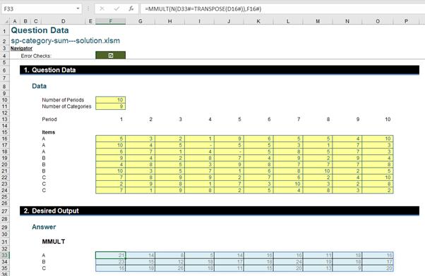
Upon completion, the outputs should resemble: 

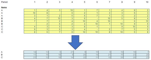
The requirements were:

• you were allowed one formula entered into one cell only
• no LAMBDA or LAMBDA helper functions (e.g. LET, BYROW or MAP) allowed
• no Power Query or VBA allowed.

Potential Solutions

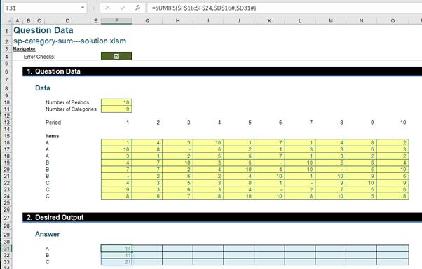
You can find our Excel file here, which shows our suggested solution.  The steps are detailed below, but first let’s look at some ways you may have tried and why they don’t work.

The most obvious way to approach this is using SUMPRODUCT.  By multiplying output category and period by the input category and period vectors we can get our answer for each individual output cell.

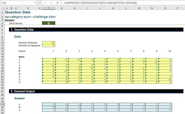
Unfortunately, this method doesn’t spill and therefore doesn’t satisfy our criteria.

Many of you may have attempted to use the SUMIFS function to sum each column by category.  The SUMIFS function requires a minimum of three arguments:

The sum_range is the range of cells to sum, the criteria_range1 is the first range being tested using criteria1 and criteria1 is the criteria being used to filter criteria_range1.  You can add as many criteria and criteria ranges as you like.

In this case, if we wanted to get a category sum for an individual row, we could use SUMIFS on the row.  The criteria range would be the list of items for the array, whilst the criteria would be the specific item we are filtering for.

Some people may be tempted to apply SUMIFS over the whole array and filter by the period as well, to try and make the whole array dynamic.  This doesn’t work as SUMIFS only works in one [1] dimension.

Our Solution

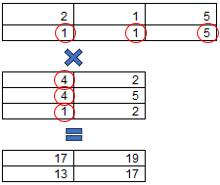
Our solution utilises the MMULT function, which is used to multiply two [2] matrices together.  Firstly, a quick refresher on how matrix multiplication works.

The output of two matrices multiplied is the height of the first matrix and the width of the second matrix.  The width of the first matrix and the height of the second matrix should be equal.  The cell outputs are found by multiplying the values in the corresponding row from the first matrix and column from the second matrix and adding the products.  For example, for the bottom left output, you take the second row of the first matrix and the first column of the second matrix: (1 x 4) + (1 x 4) + (5 x 1) = 13.

To start, we need to create a helper array.  First, we use the TRANSPOSE function on our large categories list to turn it horizontal.  By equating this to our unique categories list, we can create a helper array of 1’s and 0’s.

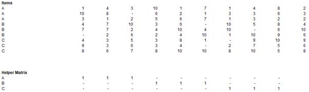
This helper array links each item row to their category.  We can actually put this inside the MMULT function and multiply it by the source array, to find the total for each category and period.

This takes each column and multiplies each value in the period by either one [1] if it’s in the category being checked, or by zero [0] if it isn’t, and adds them together, giving us just the total from that category and period.  

Can you find a shorter solution?

Word to the Wise

Just for fun, another solution can be found using the SUBTOTAL function combined with OFFSET.  To be clear, this solution is longer and unnecessarily complex, but it’s also quirky and interesting, so worth showing here.  The SUBTOTAL function can perform a range of tasks; in this case we will be using function 9 which allows us to SUM over a whole dynamic range – but unlike SUM, the calculation will spill rather than coerce.  

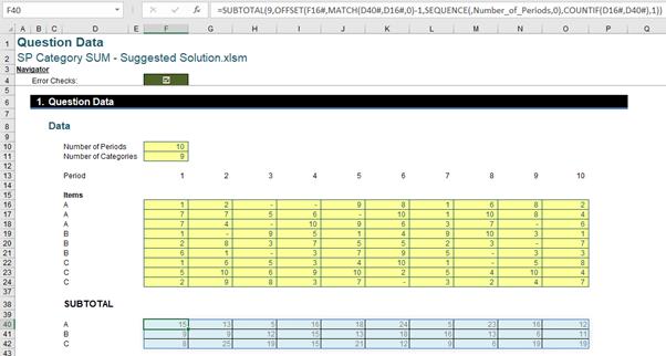
The formula we are using is:

This looks intimidating so let me break it down.  The MATCH function returns the row of the first appearance of each letter in the matrix.  Therefore, for the above, it would be {1;4;7}.  It has one [1] subtracted from it because OFFSET already starts pointing to the first row.  The COUNTIF function returns the number of rows corresponding to each letter, in this case, it is simply {3;3;3}.  The SEQUENCE function returns a list of integers growing from one [1] to the number of periods.

When we put all of this into the OFFSET function this returns three [3] times the number of periods as an array of arrays, with each position in the array containing the values that correspond to that period and that category, e.g. the top left contains the array {1;7;7}.  SUBTOTAL allows us to sum up these internal arrays and returns a spilled array of the summed values.

The Final Friday Fix will return on Friday 24 November 2024 with a new Excel Challenge.  In the meantime, please look out for the Daily Excel Tip on our home page and watch out for a new blog every business working day.