
Getting Arrays: Spilling the Beans on Seven New Functions
27 September 2018
September 24 is the day Excel moved on. Yes, we’ve had Power Pivot, Power Query / Get & Transform and Power BI, but Microsoft’s “CALC” team has been busy behind the scenes rearranging the furniture.
By “furniture” I mean the “calculation engine” – it’s had a complete re-write, and there are benefits general Excel users will reap for years to come. The first wave sees a new array calculation (“Dynamic Array”), seven new functions and two new error messages. And that’s just the start. There’s going to be plenty more coming in the next few years.
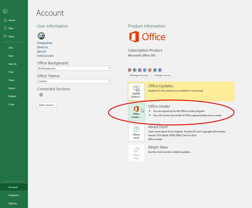
It’s all still in what Microsoft refers as “Preview” mode, i.e. it’s not yet “Generally Available” but it is something you can try and hunt out. Presently, you need to be part of what is called the “Office Insider” programme which is an Office 365 fast track. You can register in File -> Account -> Office Insider in Excel’s backstage area.
Even then, you’re not guaranteed a ticket to the ball as only some will receive the new features as Microsoft slowly roll out these features and functions. Please don’t let that put you off. These features will be with all Office 365 subscribers soon.
Let me be clear. When Office 2019 comes out, it will not include Dynamic Array functions. It’s likely you will have to wait until Office 2022 (assuming such a thing will exist) as Microsoft tries to convert everyone to the annual subscription model.
So what’s the big deal?
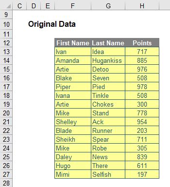
Let me begin by just looking at what a Dynamic Array is. Consider the following data:
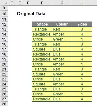
If I were to type =F12:H27 into another cell, Excel in the past would have thought I had gone mad. I’d need to wrap it in an aggregation function such as SUM, COUNT or MAX, to name but a few. Otherwise, I would have to wrap it in braces using CTRL + SHIFT + ENTER and use it as an array formula.
But no more.
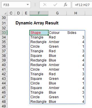
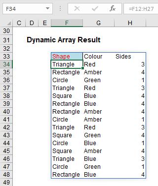
Look at what happens when I type =F12:H27 into cell F33:

The formula automatically extends to three columns by 16 rows! It has spilled. Get used to the vernacular. There’s a reason this article got the name it did!
Any formula that has the potential to return multiple results can be referred to as a Dynamic Array formula. Formulae that are currently returning multiple results, and are successfully spilling, can be referred to as Spilled Array Formulae.
Notice I did not have to highlight all of the cells F33:H48. It spilled. Also take note I formatted cell F33 – er, that didn’t spill, because presently formatting isn’t propagated. This is why this is not yet Generally Available. Microsoft is still trying to work out what should and shouldn’t be allowed to happen in this first release. But don’t let that put you off.
And don’t let this basic example put you off either. If you feel a general sense of underwhelm coming over you, it’s because I haven’t yet communicated how powerful this all is as my example was too basic.
However, before I carry on there is a question I do need to cover with my far too simple example: what happens if something gets in the way?
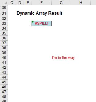
In this example, in cell G40, I have typed in the obtrusive text, “I’m in the way”. And it quite literally is. Consequently, I have generated the brand new #SPILL! error. The formula cannot spill, so the error message is generated accordingly.
#SPILL! Errors
#SPILL! errors are returned when a formula returns multiple results, and Excel cannot return the results to the spreadsheet. There are various reasons an #SPILL! error could occur:
- spill range is not blank: as in my example (above), this error occurs when one or more cells in the designated spill range are not blank and thus may not be populated.
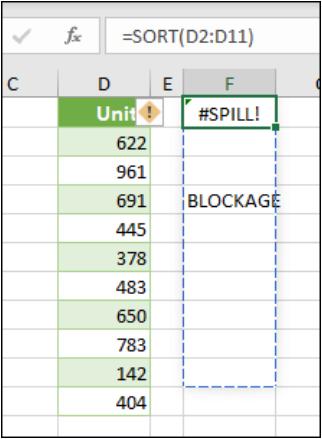
When the formula is selected, a dashed border will indicate the intended spill range. You may select the error “floatie” (believe it or not, this is what Microsoft call these things!), and choose the ‘Select Obstructing Cell’ option to immediately go the obstructing cell. You can then clear the error by either deleting or moving the obstructing cell's entry. As soon as the obstruction is cleared, the array formula will spill as intended
the range is volatile in size: this means the size is not “set” and can vary. Excel was unable to determine the size of the spilled array because it's volatile and resizes between calculation passes. For example, the new function SEQUENCE(x) (explained in detail below) generates a list of x numbers increasing by 1 from 1 to x. That’s fine, but the following formula will trigger this #SPILL! error:
=SEQUENCE(RANDBETWEEN(1,1000)).
- Dynamic array resizes may trigger additional calculation passes to ensure the spreadsheet is fully calculated. If the size of the array continues to change during these additional passes and does not stabilise, Excel will resolve the dynamic array as #SPILL! This error type is generally associated with the use of RAND, RANDARRAY and RANDBETWEEN functions. Other volatile functions such as OFFSET, INDIRECT and TODAY do not return different values on every calculation pass so tend not to generate this error
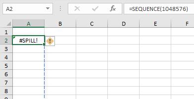
- extends beyond the worksheet’s edge: in this situation, the spilled array formula you are attempting to enter will extend beyond the worksheet's range. You should try again with a smaller range or array. For example, moving the following formula to cell A1 will resolve the error, and the formula will spill correctly
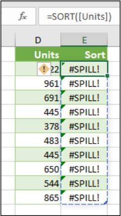
- Table formula: as I will explain shortly, Tables and Dynamic Arrays are not yet best friends. Spilled array formulae aren't supported in Excel Tables (generated by CTRL + T). Try moving your formula out of the Table, or go to Table Tools -> Convert to range
- out of memory: I have forgotten what this one means. Sorry, I couldn’t resist that. The spilled array formula you are attempting to enter has caused Excel to run out of memory. You should try referencing a smaller array or range
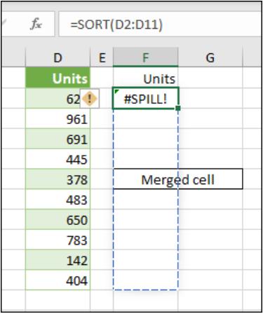
- spill into merged cells: spilled array formulae cannot spill into merged cells. You will need to un-merge the cells in question or else move the formula to another range that doesn't intersect with merged cells.
- When the formula is selected, a dashed border will indicate the intended spill range. You can again select that wonderfully named error floatie and choose the ‘Select Obstructing Cell’ option to immediately go the obstructing cell. As soon as the merged cells are cleared, the array formula will spill as intended
- unrecognised / fallback error: the “catch all” variant. Excel doesn't recognise, or cannot reconcile, the cause of this error. Here, you should make sure your formula contains all of the required arguments for your scenario.
Returning to Dynamic Arrays
Now that we have considered what happens if you block a Dynamic Array, let me now turn my attention to what happens if you don’t. You get the following:
Do you see I am not having to anchor cells (i.e. use dollar [$] signs)? The formula just spills. Let me be clear. If I select cell F34, I get the following:
Here’s a first. Check out the formula in the formula bar. It’s greyed out. Ever seen that before? Effectively, cell F34 contains the value ‘Triangle’ but it does not actually contain an “Excel” formula in the usual sense. To demonstrate this, let me show you the VBA Immediate Window:
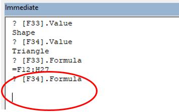
But, to quote Bill Jelen, similar to Schrodinger's Cat, if you select cells F33:H48 and use ‘Go To Special’ (F5 -> Special), and then select ‘Formulas’, cells F33:H48 are shown as formula cells. You can even copy and paste them as values. Ladies and gentlemen, welcome to The Twilight Zone (cue eerie music).
I mentioned in the #SPILL! errors section that you cannot use Dynamic Arrays in a Table, but Dynamic Arrays may refer to a Table, viz.
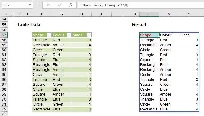
In this above illustration, cells F57:H72 have been converted into a Table (CTRL + T), with the Table named Basic_Array_Example. In cell L57, I have simply typed ‘=’ and then highlighted the entire Table. It was all replicated.
The advantage of linking a Dynamic Array to a Table is clear:
I can add rows and / or columns and the Dynamic Array will update automatically. Do note that this does not breach the #SPILL! range is volatile in size error. This is because the range size will not vary on every calculation pass.
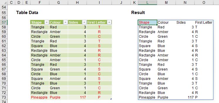
Talking of varying sizes, it’s clear to see one potential issue with Dynamic Arrays. If we are not referring to a Table, what happens if the source data changes dimensions? This may be why you should refer to a Table for safety.
However, once you have a Dynamic Array, referring to it is simple using what is known as the Spilled Range Operator. For example, if I want to refer to the Dynamic Array in the previous examples, it initially had a range of L57:N72. However, once I had added a row and column to the Table, this resized to L57:O73. I can easily refer to this array, whatever its size as follows. In its initial state:
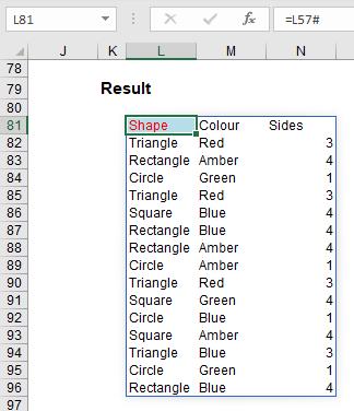
The formula =L57# allows for variations – you simply type in the top left-hand cell reference (i.e. the cell with the non-greyed out formula) and add ‘#”, known as the Spilled Range Operator. Simple!
It’s not all peaches and cream though. Whilst Dynamic Arrays and Tables share some similarities, they are very different beasts. This couldn’t be clearer than when you create charts:

Here, I created two charts when I only had the data up to June. Then, I added the data for July. The chart on the left referencing the Table source data updated instantly. However, the chart on the right still only displayed up to June even though the Dynamic Array had updated.
Conclusion: use Tables, not Dynamic Arrays, as your references for dynamic charts.
Implicit Intersection Implications
It may be an alliteration and sound like something you can get arrested for, but Dynamic Arrays do come at a price. There aren’t many users out there who used them, but there are some – and hence there will be some legacy calculations affected.
In the past, if you entered =A$1:A$10 anywhere in rows 1 through 10, the formula would return only the value from that row. In fact, a spreadsheet our company is presently auditing relies on this behaviour. However, in the brave new world of Office 365 (albeit selected Insider recipients for the time being), typing this formula would create a Spilled Array Formula. To protect existing formulae, we need a new – if not instantly breathtaking – function…
SINGLE Function
Don’t judge the remaining six functions on our first newbie. This one is essential to keep Excel running smoothly, but it’s probably safe to say it won’t set the world alight. It’s like toilet roll – imagine your situation without it…
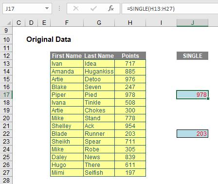
The SINGLE function returns a single value using logic known as implicit intersection. SINGLE may return a value, single cell range or an error.
The function has the following syntax:
=SINGLE(value).
The function has just one argument:
- value: this argument is required and represents the array to be selected.
When the supplied argument is a range, SINGLE will return the cell at the intersection of the row or column of the formula cell. Where there is no intersection, or more than one cell falls in the intersection, then SINGLE will return a #VALUE! error. When the supplied argument is an array, SINGLE returns the first item (Row 1, Column 1).
In the example below, the two SINGLE formulae are supplied a range, H13:H27, and return the values in cells H17 and H22 respectively.
I can see an argument going forward that some form of OFFSET (e.g. “NEXT” or “PRIOR”) may be needed in due course – but no one is expecting everything to come together on Day 1.
Dynamic Arrays vs. Legacy Array Formulae
Prior to this new functionality, if you wanted to work with ranges in Excel, you used to have to build array formulae, where references would refer to ranges and be entered as CTRL + SHIFT + ENTER formulae. The main differences are as follows:
- Dynamic Array formulae may spill outside the cell bounds where the formula is entered. The Dynamic Array formula technically only exists in the cell in the top left-hand corner of the spilled range (as shown earlier), whereas with a legacy CTRL + SHIFT + ENTER formula, the formula would need to be entered in the entire range
- Dynamic arrays will automatically resize as data is added or removed from the source range. CTRL + SHIFT + ENTER array formulae will truncate the return area if it's too small, or return #N/A errors if too large
- Dynamic array formulae will calculate in a 1 x 1 context
- Any new formulae that return more than one result will automatically spill. There's simply no need to press CTRL + SHIFT + ENTER
- According to Microsoft, CTRL + SHIFT + ENTER array formulae are only retained for backwards compatibility reasons. Going forward, you should use Dynamic Array formulae instead
- Dynamic array formulae may be easily modified by changing the source cell, whereas CTRL + SHIFT + ENTER array formulae require that the entire range be edited simultaneously
- Column and row insertion / deletion is prohibited in an active CRL + SHIFT + ENTER array formula range. You first need to delete any existing array formulas that are in the way.
Everybody clear? I think we are finally good to start introducing the other new functions…
SORT Function
I am not going to do these alphabetically – let me show then in an order that makes sense (well, to me, anyway).
The SORT function sorts the contents of a range or array:
=SORT(array, [sort_index], [sort_order], [by_column]).
It has four arguments:
- array: this is required and represents the range that is required to be sorted
- sort_index: this is optional and refers to the position of the row or the column in the selected array (e.g. second row, third column). 99 times out of 98 you will be defining the column, but to select a row you will need to use this argument in conjunction with the fourth argument, by_column. And be careful, it’s a little counter-intuitive! The default value is 1
- sort_order: this is also optional. The choices for sort_order are 1 for ascending (default) or -1 for descending. It should be noted that you might not want to hold your breath waiting for ‘Sort by Color’ (sic), ‘Sort by Formula’ or ‘Sort by Custom List’ using this function
- by_column: this final argument is also optional. Most people want to sort rows of data, so they will want the value to be FALSE (which is the default value if not specified). Should you be booking your mental health check, you may wish to use TRUE to sort by column in certain instances.
This is a function people have been crying out for, for years. Enterprising spreadsheets gurus have developed array formulae and user-defined functions that have replicated this functionality, but you don’t need it anymore! SORT is coming to a theatre near you very soon.
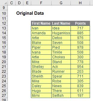
To show you how devilishly simple it is, consider the following data:
Sorting the ‘Points’ column in order is easy as this:
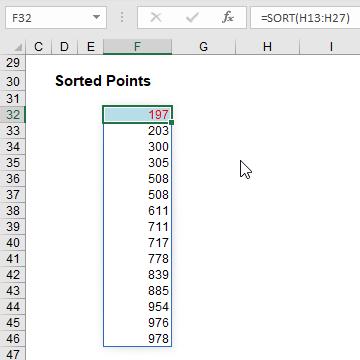
All you have to do is type =SORT(H13:H27) into cell F32. That’s it! Note that the duplicates are repeated; there is no cull. If you want it in descending order, simply specify the requirement in the formula:
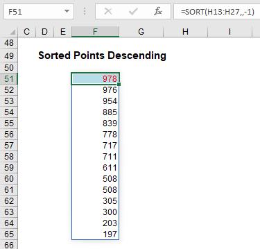
This formula is only slightly more sophisticated, in that the sort_order (third argument) needs to be specified as -1 to switch the sort to descending:
=SORT(H13:H27,,-1).
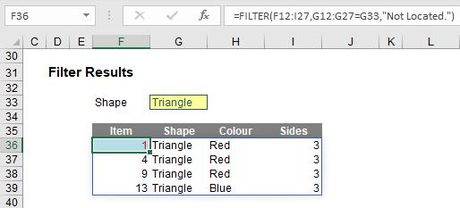
You probably won’t want the points displayed on their own:
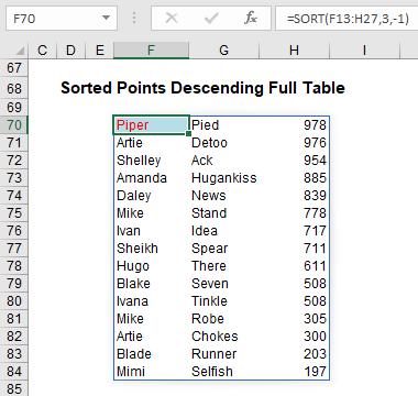
Now all of these arguments start to make more sense. SORT(F13:H27,3,-1) produces the whole array (array is F13:H27), sorts it on the third (sort_index 3) column in descending (sort_order -1) order. Blake and Ivana tie on 508 points, but Blake appears first as he was first in the original (source) table.
So far, I have only performed the one SORT. You can have more than one though:
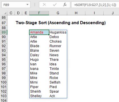
Here, I have created a second (two-level) SORT. Here, you need to create what is known as an array constant for the second and third arguments (you just type the braces in – don’t use CTRL + SHIFT + ENTER):
=SORT(F13:G27,{1;2},{1;-1}).
This will sort on column 1 (‘First Name’) first, then sort on column 2 (‘Last Name’) next. This will be in ascending order (1) for the first column and descending order (-1) for the latter. It’s not as straightforward a formula entry as most Excel modellers are used to, but it’s relatively straightforward once you have committed it to erm, um, what do you call it, memory.
My final example of SORT is not something that is limited to this new function, but it does show how things fit together. From all that has been written above, it appears you can only get one value (using SINGLE) or all of them (using Dynamic Arrays). That’s not true as this illustration clearly demonstrates:
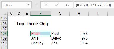
Only the top three have spilled in this example. How? Well, I cheated. I highlighted cells F108:H110 first, then typed in the formula
=SORT(F13:H27,3,-1)
and then pressed CTRL + SHIFT + ENTER (thus generating the { and } braces). This restricted the spill to the range stipulated. Cool. Other than making sure no one can delete or insert any rows by creating an array formula such as {=1} across the restricted area, these appear to be the only two used of CTRL + SHIFT + ENTER now.
SORT is really useful then, but what if you want to sort on a field you don’t want displayed in the results..?
SORTBY Function
The SORTBY function sorts the contents of a range or array based on the values in a corresponding range or array, which does not need to be displayed. The syntax is as follows:
=SORTBY(array, by_array1, [sort_order1], [by_array2], [sort_order2], …).
It has several arguments:
- array: this is required and represents the range that is required to be sorted
- by_array1: this is the first range that array will be sorted on and is required
- sort_order1, sort_order2, …: these are optional. The choices for each sort_order are 1 for ascending (default) or -1 for descending
- by_array2, …: these arguments are also optional. These represent the second and subsequent ranges that array will be sorted on.
There are some important considerations to note:
- the by_array arguments must either be one row high or one column wide
- all of the by_array arguments must be the same size and contain the same number of rows as array if sorting on rows, or the same number of columns as array if sorting on columns
- if the sort order argument is not 1 or -1, the formula will result in a #VALUE! error.
It’s pretty simple to use. Consider the following source data once more:
I can use SORTBY as follows:
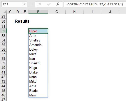
Here, using the formula
=SORTBY(F13:F27,H13:H27,-1,G13:G27,1)
I have sorted the ‘First Name’ field (F13:F27) on the ‘Points’ column (H13:H27) in descending (-1) order and then used the second sort on ‘Last Name’ (G13:G27) in ascending (1) order. No need for those pesky array references in multiple sorts with the SORT function (as detailed above).
FILTER Function
The FILTER function will accept an array, allow you to filter a range of data based upon criteria you define and return the results to a spill range.
The syntax of FILTER is as follows:
=FILTER(array, include, [if_empty]).
It has three arguments:
- array: this is required and represents the range that is to be filtered
- include: this is also required. This specifies the condition(s) that must be met
- if_empty: this argument is optional. This is what will be returned if no data meets the criterion / criteria specified in the include argument. It’s generally a good idea to at least use “” here.
For example, consider the following source data:
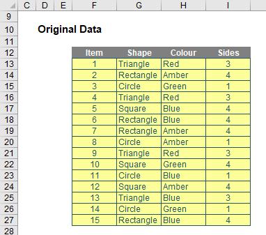
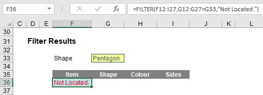
To begin with, I will perform a simple FILTER:
Here, in cell F36, I have created the formula
=FILTER(F12:I27,G12:G27=G33,”Not Located.”)
F12:I27 is my source array and I wish only to include shapes (column G12:G27) that are ‘Triangles’ (specified by cell G33). If there are no such shapes, then “Not Located.” is returned instead. To show this, I will change the shape as follows:
That is about as basic as it gets. I can get cleverer. Consider the following example:
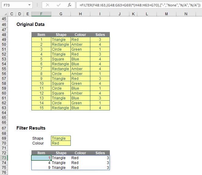
I have repeated the source array (cells F48:I63) for clarity. The formula
=FILTER(F48:I63,(G48:G63=G69)*(H48:H63=G70),{"-","None","N/A","N/A"})
looks horrible to begin with, but it’s not quite as bad as it appears upon further scrutiny. The include argument,
(G48:G63=G69)*(H48:H63=G70)
contains two conditions. Firstly, G48:G63=G69 means that the ‘Shape’ (column G48:G63) has to be a ‘Triangle’ (cell G69) and that the ‘Colour’ (column H48:H63) has to be ‘Red’ (cell G70). The multiplication operator (*) is used to denote AND. The Excel function AND cannot be used with arrays – this is nothing special to Dynamic Arrays; AND does not work with CTRL + SHIFT + ENTER formulae either. This syntax is similar to how you would create AND criteria with the SUMPRODUCT function, for example.
The final argument is similar to the syntax in SORT: {"-","None","N/A","N/A"}. Braces (typed in!) are used to create an array argument that specifies what should be written in each column should there be no record that meets both criteria, e.g.
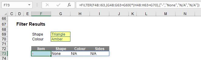
See? Not as bad as you might first think.
My final example is very similar:
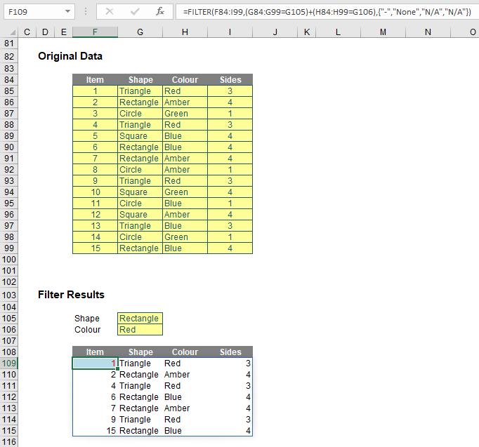
Once you realise I have simply repeated referencing for clarity, the formula
=FILTER(F84:I99,(G84:G99=G105)+(H84:H99=G106),{"-","None","N/A","N/A"})
is nothing more than the OR equivalent of the previous example, with ‘+’ replacing ‘*’ to switch from ensuring both conditions are met to only one condition being met. As at the time of writing, XOR is not catered for, but I am sure some clever person will create an equivalent in due course (if Microsoft doesn’t beat them to it), necessity being the mother of invention and all that jazz.
Interlude: the #CALC! Error
I mentioned there were two new error messages. I have only referred to #SPILL! so far. There is another, lurking in the background (I say “in the background” as at the time of writing, Microsoft hasn’t written any documentation on it!).
Sometimes, as you explore how you can combine Excel functions with each other you get error messages (e.g. more often than not trying FILTER(FILTER(… will generate an #VALUE! error). When you start playing with these new array functions, you might stumble upon #CALC! This is a new one.
To add to the myriad of error messages such #REF!, #DIV/0!, #VALUE!, #BROWN and #PIPE, let’s introduce #CALC! – which probably means something like, "Excel cannot currently figure out the answer presently, but might be able to in a future release, no promises though". I look forward to the documentation in due course though to fathom its real meaning (probably something like, “Help! Abandon ship!”).
Let’s move on.
UNIQUE Function
The hilarious thing about UNIQUE is that it does two things (!). It details distinct items (i.e. provides each value that occurs with no repetition) and also it can return values which occur once and only once in a referred range. I understand that Excel users may welcome the former use with open arms and that database developers may be very interested in the latter. I still think there should have been two functions though. Otherwise, let’s just extend the >AGGREGATE function to do just everything (it almost does now) and be done with it!
The UNIQUE function has the following syntax:
=UNIQUE(array, [by_column], [occurs_once]).
It has three arguments:
- array: this is required and represents the range or array from which to return unique values
- by_column: this argument is optional. This is a logical value (TRUE / FALSE) indicating how to compare. If you wish to compare by row, the argument should be FALSE or omitted (since this is the default). To compare by column, you will need to select TRUE
- occurs_once: this argument is also optional. This requires a logical value too:
- TRUE: only return unique values that occur once
- FALSE: include all distinct values (default if omitted).
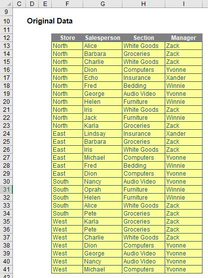
It’s probably clearer with some examples. Let’s give it a go. As always, I need source data:
Time for the most basic illustration:
In cell L13, I have simply typed
=UNIQUE(F13:F41).
No optional arguments; everything in default. If I have made an error, it’s going to be my default. This has simply listed each store that appears; if “North” and “North ” (extra space) were there, then both would appear. UNIQUE is not case sensitive though and each entry would appear as it first occurs reading down the range F13:F41. The other columns contain similar formulae and UNIQUE looks like it takes seconds to learn. Presently, there’s an in-joke going around the Excel Most Valuable Professionals (MVPs) that array expert Mike Girvin is going to be choked as he dedicated an entire chapter in one of his books to creating that list with an array formula! Sorry Mike. Excel is fun!
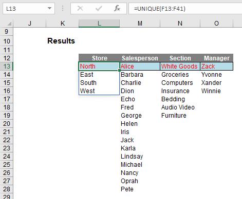
It’s just as simple if you want to see unique records for two (or more) columns, viz.
You can see UNIQUE is sort of crying out for SORT, but we’ll get to that shortly.
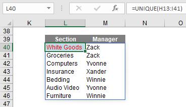
As mentioned earlier, it’s not the only way of using UNIQUE (no, having a unique use would be just what “they” were expecting, whoever “they” are…). You can use it to determine values that only occur once:
Here, the formula in cell L56,
=UNIQUE(G56:G84,0,1)
uses the non-default value of 1 for the optional occurs_once (third) argument. This means it identifies the salespeople who only occur once in cells G56:G84. Brilliant; I can die content knowing now.
The real power starts coming when you start playing with Excel’s existing functions and features, together with these new functions. Take this comprehensive example:
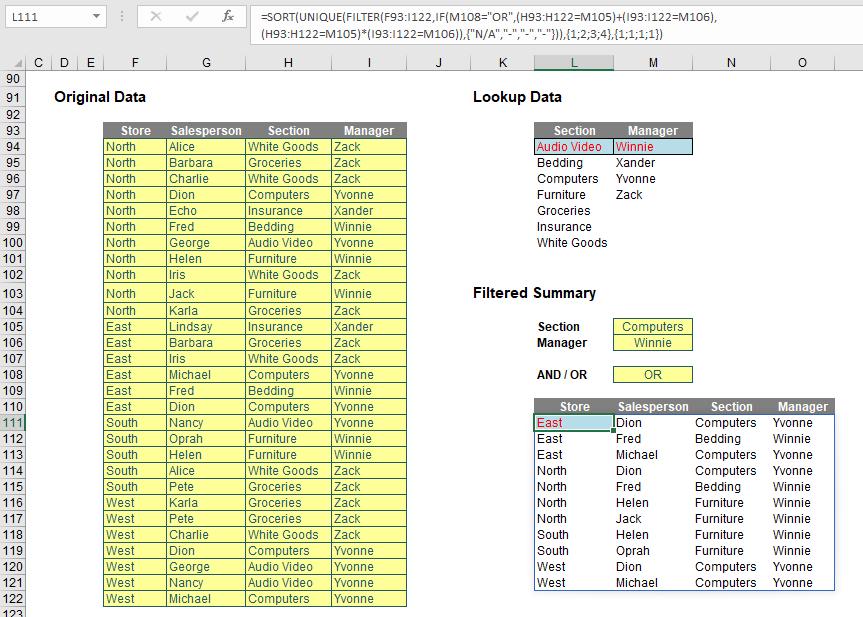
Let me step you through some of this. The formulae in cells L94 and M94 use UNIQUE in a similar manner to my first example, to generate the list of distinct values in the ‘Section’ and ‘Manager’ fields. However, did you notice they have been sorted? That’s because I used the formula
=SORT(UNIQUE(H94:H122))
in cell L94, for example. Honestly, I think UNIQUE should have another argument for sorting (ascending / descending / none [default]). Watch Microsoft ignore that suggestion.
But then I did something really cool. Cells M105 and M106 use data validation (ALT + D + L) to generate a list from the ‘Lookup Data’ section. That requires taking a closer look:
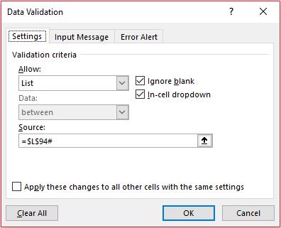
Do you see the source for the data validation in cell M105? =$L$84# - so elegant! This takes the ‘Section’ list and automatically makes the drop-down list the required length! People create all sorts of tricks using OFFSET, dynamic range names and the like to achieve a similar effect. No more. =$L$84# (with the ‘#’, the Spilled Range Operator) is all that is needed. That’s my favourite thing in all of these new functions and features. I’m impressed – and I’m easily impressed.
The ‘AND / OR’ dropdown is a bit of an anti-climax after that, but the final formula that generates the final table, namely
=SORT(UNIQUE(FILTER(F93:I122,IF(M108="OR",(H93:H122=M105)+(I93:I122=M106),
(H93:H122=M105)*(I93:I122=M106)),{"N/A","-","-","-"})),{1;2;3;4},{1;1;1;1})
is rather fun. I am not going to go through it though – as every aspect of this formula is simply a re-hash of an earlier point (assuming you know the IF function!). See if you can work your way through it for yourself.
SEQUENCE Function
The penultimate function is SEQUENCE. This function allows you to generate a list of sequential numbers in an array, such as 1, 2, 3, 4. It doesn’t sound particularly exciting, but again, it really ramps up when combined with other functions and features. The syntax is given by:
=SEQUENCE(rows, [columns], [start], [step]).
It has four arguments:
- rows: this argument is required and specifies how many rows the results should spill over
- columns: this argument is optional and specifies how many columns (surprise, surprise) the results should spill over. If omitted, the default value is 1
- start: this argument is also optional. This specifies what number the SEQUENCE should start from. If omitted, the default value is 1
- step: this final argument is also optional. This specifies the amount each number in the SEQUENCE should increase (the “step”). It may be positive, negative or zero. If omitted, the default value is 937,444. Wait, I’m kidding; it’s 1. They’re very unimaginative down in Redmond.
Therefore, SEQUENCE can be as simple as SIMPLE(x), which will generate a list of numbers in a column 1, 2, 3, …, x. Therefore, be mindful not to create a formula where x may be volatile and generate alternative values each time it is calculated, e.g. =SEQUENCE(RANDBETWEEN(10,99)) as this will generate the #SPILL! range is volatile in size error.
A vanilla example is rather bland:
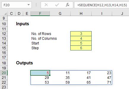
Do you see how SEQUENCE propagates across the row first and then down to the next row, just like reading a book? I wonder how that might work in alternative languages of Excel where users read right to left (it has to be the same or there would be chaos when workbooks were shared!).
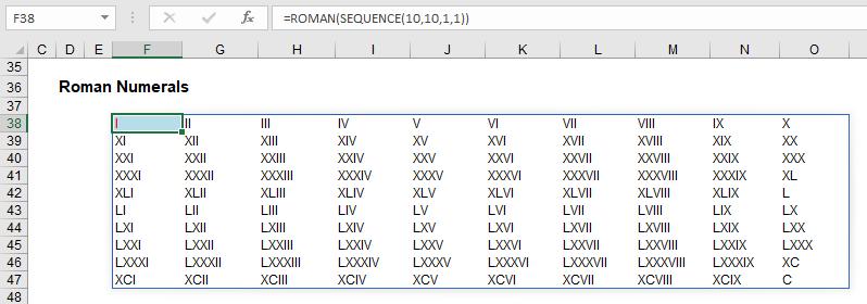
Some of my peers had fun combining it with the ROMAN function:
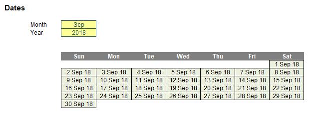
To my mind though, my favourite simple illustration is creating a monthly calendar. A little magic with the DATE and WEEKDAY functions combined with some conditional formatting and suddenly you have:
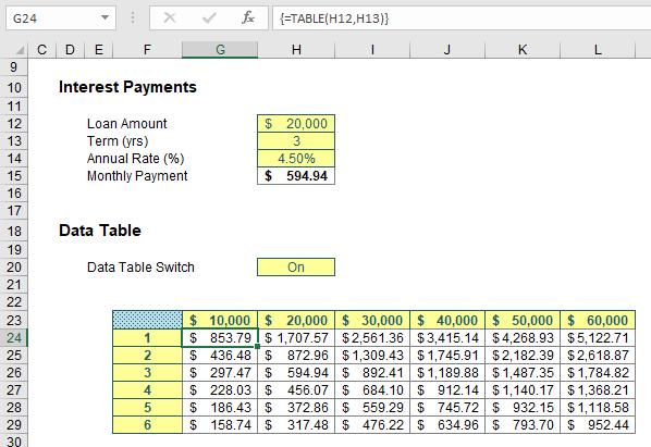
As I mentioned above, SEQUENCE is arguably more powerful when included in a more complex formula. For example:
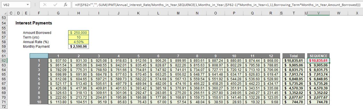
In this instance, I have created a grid using the Excel IPMT function to determine the amount of interest to be paid in each monthly instalment. Cells G62:R71 calculate each monthly amount and column T sums these amounts to calculate the annual interest payment, a figure which is non-trivial to compute. The whole table may be replaced by the formula in cell V62:
=IF($F62="","",-SUM(IPMT(Annual_Interest_Rate/Months_in_Year,
SEQUENCE(1,Months_in_Year,($F62-1)*Months_in_Year+1,1),
Borrowing_Term*Months_in_Year,Amount_Borrowed))).
I am not going to explain this and let me tell you why. Our company, SumProduct builds and reviews financial models for a living. We see terrible modelling practices established day-in, day-out. We proactively try to discourage these traits by emphasising that complex formulae should be stepped out and made transparent. Here, that can be done using the original table. I don’t want people using SEQUENCE, Dynamic Arrays or other spilled formulae to wrap up complicated calculations into an opaque Pandora’s Box. Yes, calculation times may be slower. Live with it. Sometimes you need to see the scenery to appreciate the beauty. I’m just a little fearful that people will embrace these functions a little too readily and the Road to Excel Hell beckons shortly. Sorry to be a miserable git.
On an upbeat note, I put a formula in cell G61 which is simple:
=TRANSPOSE(SEQUENCE(Months_in_Year)).
Yes, I am using TRANSPOSE without CTRL + SHIFT + ENTER. We are in new territory here…
RANDARRAY Function
And so, to the final function for now: RANDARRAY. The RANDARRAY function returns an array of random numbers between 0 and 1. It’s not clear from Microsoft, but it’s my belief this is analogous to the pre-existing RAND function, which generates a number greater than or equal to zero and strictly less than one. It is noted though that RANDARRAY is different from the RAND function insofar that RAND does not return an array.
The function has the following syntax:
=RANDARRAY([rows], [columns]).
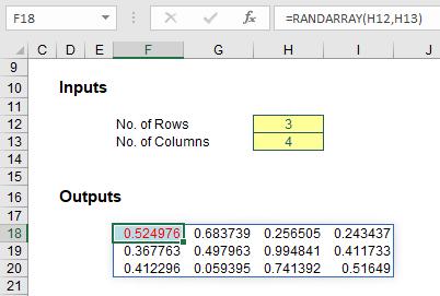
The function has two arguments, both optional:
- rows: this specifies how many rows the results should spill over. If omitted, the default value is 1
- columns: this specifies how many columns the results should spill over. If omitted, the default value is also 1.
Therefore, RANDARRAY() behaves like RAND().
Again, I’ll start with a basic demonstration:
This can be useful for generating “seed” values for simulations analysis, for example. Anecdotal evidence suggests using RANDARRAY in a simulations formula rather than using a macro or Data Table may generate calculation speed efficiencies of greater than 50%. The jury is still out on this one – but it’s definitely worth exploring.
There is no RANDBETWEENARRAY function, but you can construct it yourself:
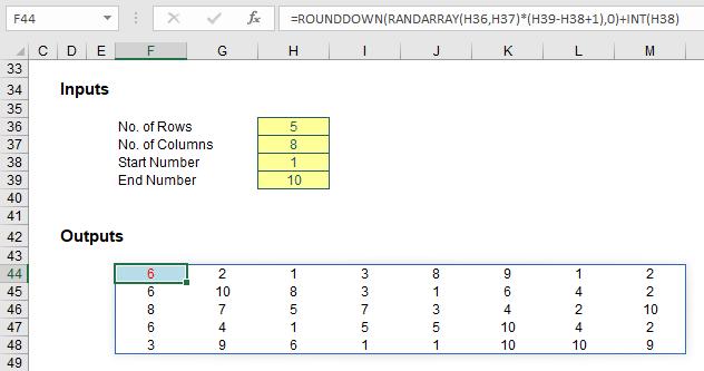
Here, in cell F44, I have used the formula
=ROUNDDOWN(RANDARRAY(H36,H37)*(H39-H38+1),0)+INT(H38)
to generate my equivalent RANDBETWEEN function. Since RANDARRAY generates a random number greater than or equal to zero and strictly less than one, ROUNDDOWN(RANDARRAY(H36,H37)*(H39-H38+1),0) generates a random integer (all equally likely) between zero and nine (this is 9, because the number generated is a whole number greater than or equal to zero but strictly less than 10 [10 – 1 + 1]). Since this is added to 1 (INT(H38)), the random whole number will be an integer between 1 and 10. Simple, if you have a Maths PhD.
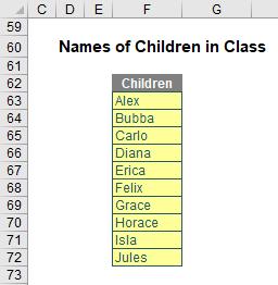
For a final example, imagine you are a schoolteacher and you have 10 five-year-old children:
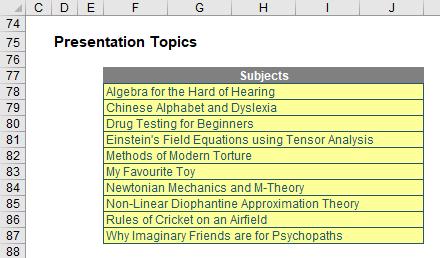
For each of the next 10 weeks, you have topics you want one of them to present on:
I can use RANDARRAY in tandem with SORTBY to determine a presentation order for the term:
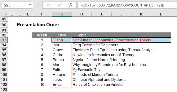
Oh dear. I do hope Diana has prepared well or it could all end in tears. She could try swapping with Horace, I suppose. On a serious note, the formula
=SORTBY(F63:F72,RANDARRAY(COUNTA(F63:F72)))
sorts the ‘Child’ order randomly (and a similar formula is used for ‘Topic’ too). In a past life, as an independent expert, I once had to attest that drug testing was being performed entirely randomly, i.e. free from any material bias. SORTBY(RANDARRAY) dries up that well for me once and for all.
Death of Data Tables and PivotTables?
I near the end of this rather long article on an interesting note or two. There are some significant ramifications for Excel, once these functions and features roll out and become Generally Available (this does assume the “final” versions of everything highlighted here do not change drastically).
Let me explain.
I begin with a two-dimensional Data Table (ALT + D + T) with an old favourite for this sort of thing, calculating monthly payments on various loan amounts over various durations.
I have no plans to go through Data Tables here, suffice to say they are a great tool for “what-if?” analysis, albeit they can consume vast quantities of memory. This summary table shows how the monthly instalments would vary for different terms (in years) and different amounts borrowed.
Now, take a look at using three Dynamic Array formulae:
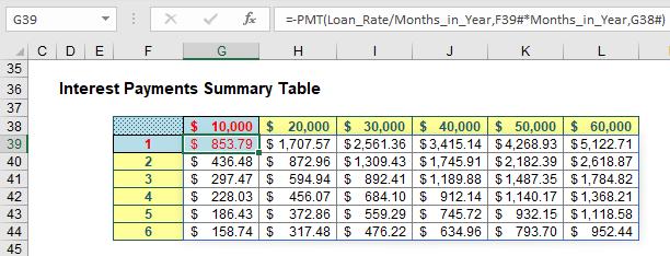
Can you spot the difference? In the second table, I have highlighted three cells:
- G38 contains the formula =SEQUENCE(1,6,10000,10000)
- F39 contains the formula =SEQUENCE(6)
- G39 contains the formula =-PMT(Loan_Rate/Months_in_Year,F39#*Months_in_Year,G38#). See how using the Spilled Range Operator (‘#’) makes all the difference?
That’s it! Now I am not saying all Data Tables may be replaced by Dynamic Array formulae, but can you see the future? And guess what, it doesn’t stop there. Let me replicate one feature in Excel many of us are familiar with: the PivotTable…
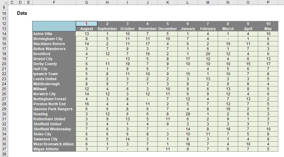
In this illustration, I have created a 1,200-record Table (CTRL + T):
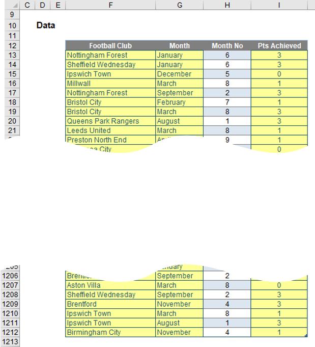
It’s all made up randomly generated data, and you will just have to guess who I support. The important thing to note is I have created a Table, called Football_Data, so I may add records and the Table will extend automatically.
Next, I created a “Pseudo PivotTable”:
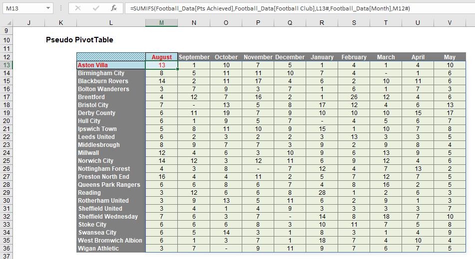
This was created using three Dynamic Array formulae (again, highlighted):
- M12 contains the formula =TRANSPOSE(UNIQUE(SORTBY(Football_Data[Month],Football_Data[Month No]))), which sorts the months into the required order
- L13 contains the formula =SORT(UNIQUE(Football_Data[Football Club])), which simply sorts the clubs into alphabetical order
- M13 contains the formula =SUMIFS(Football_Data[Pts Achieved],Football_Data[Football Club],L13#,Football_Data[Month],M12#), which spills out the points earned each month using a standard SUMIFS formula and the Spilled Range Operator (‘#’).
Think about it. I have created a formulaic PivotTable which calculates no discernibly slower than the real thing. However, the source data may be extended, values may change and I don’t need to hit ‘Refresh’. Is this the end for PivotTables?
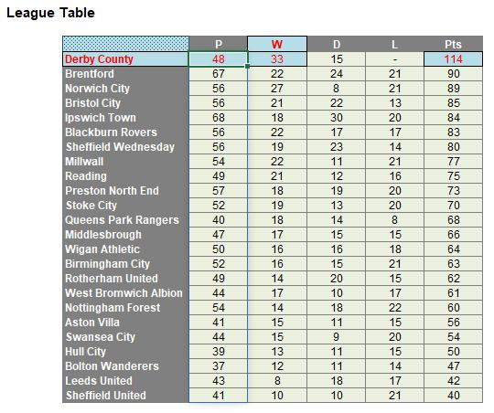
It’s easy to get carried away. Dynamic Array formulae make league tables a breeze:
However, rather than get side tracked, I’d rather stay “on track” with PivotTables and finish this section unpivoting the PivotTable we have just created (the references have changed as they are on a different worksheet in my example):
Unpivoting can be a nightmare, but it is possible. You don’t need to use Dynamic Arrays to do it, but I will to showcase them:
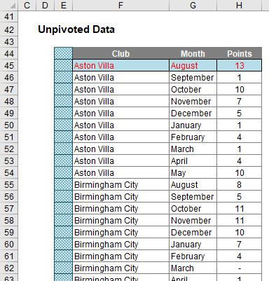
There is a hidden formula in cell E45. You can see why it is hidden – for those of you with a nervous disposition, please look away now:
=INDEX(SORT(G12#&" - "&F14:F37),ROUNDUP(SEQUENCE(COUNTA(F14:F37)
*COUNT(G12#))/COUNT(G12#),0),MOD(SEQUENCE(COUNTA(F14:F37)*COUNT(G12#))
-1,COUNT(G12#))+1).
Oh dear. That’s a horror. Rather than write 1,000 words trying to explain this, let me detail the concept instead. SORT(G12#&" - "&F14:F37) provides every combination of Month Number concatenated with a Football Club, separated by a “ – “ delimiter, e.g.
1 – Aston Villa, 2 – Aston Villa, …, 10 – Aston Villa, 1 – Birmingham City, 2 – Birmingham City, …
The problem is SORT(G12#&" - "&F14:F37) spills this into a 10-column by 24-row array. I want it as a list, so the entire rest of the formula simply forces the array down a column of 240 rows instead. INDEX is used to locate the next record in the array, with contrived formulae to determine the row and column numbers of the virtual grid.
SUMIFS is used to create the points total for each row, and to be honest, simpler formulae could have been used elsewhere too. But that’s my point. As I have written this article, it’s hard not to get carried away with all this and try and do everything in Dynamic Arrays. I have worked for years with Excel and been a keen advocate for keeping everything simple. Dynamic Arrays scare me that we may not help ourselves and write monsters like the formula above.
Maybe Excel’s simpler functions and features will live on after all.
Calculation Order Concern
If it feels like you have aged a year since you started reading this, you probably have. There’s a lot to get excited about and I have highlighted some of the issues too – many of which I am sure will be ironed out by the time everything becomes Generally Available. However, I am not sure the following concern will be going away any time soon.
When I calculate something in Excel, if I use the same formula, I must get the same answer, right? Well – not necessarily. Consider the following:
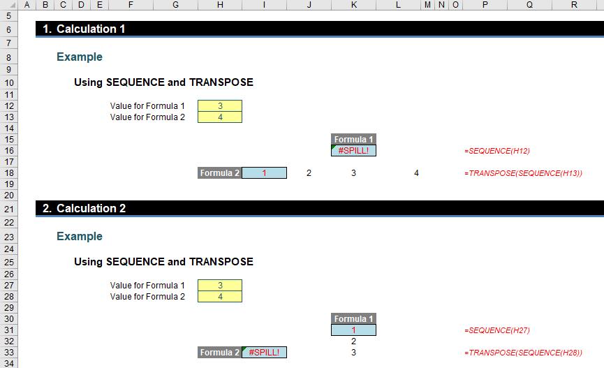
In the example above, Calculations 1 and 2 are identical but deliver different results (i.e. different #SPILL! errors). Why?
- In Calculations 1 and 2, both values for Formula 1 and Formula 2 were originally set to 1. This causes no #SPILL! errors
- In Calculation 1, the value for Formula 2 (cell H13) was then changed to 4 with no error
- Then, in Calculation 1, the value for Formula 1 (cell H12) was changed to 3. This caused the resultant #SPILL! error in cell K16
- Next, in Calculation 2, the value for Formula 1 (cell H27) was changed to 3 with no error
- Then, in Calculation 2, the value for Formula 2 (cell H28) was changed to 4. This caused the resultant #SPILL! error in cell I33.
I am not sure what the solution is for this problem. Technically, #SPILL! is working correctly, but it doesn’t seem right that two results may be generated in this instance depending upon what input I change first. The jury is out on this one.
Word to the Wise
As at the time of writing, all the features, functions and error messages are beta features only. They are available to a portion of Office Insiders at this time, but don’t let that put you off. Start getting excited now! Microsoft will continue to optimise these features over the next several months. This means they might change. When they're fully cooked, Microsoft will release them out into the wild, first to all Office Insiders and then finally Office 365 subscribers (this is when a feature is known as “Generally Available”).
The future’s looking bright though. In the meantime, feel free to download the attached Excel file, but please note you may receive a workbook full of errors if you don't have the right version of Excel!