
A to Z of Excel Functions: The MMULT Function
4 July 2022
Welcome back to our regular A to Z of Excel Functions blog. Today we look at the MMULT function.
The MMULT function
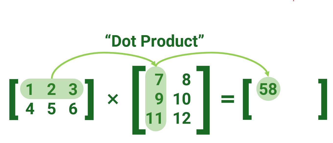
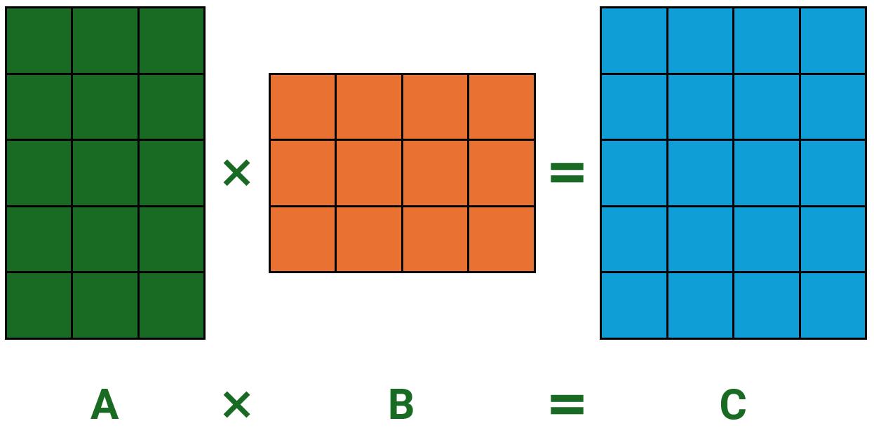
In mathematics, matrix multiplication is what’s known as a binary operation that produces a matrix from two matrices. For matrix multiplication, the number of columns in the first matrix must be equal to the number of rows in the second matrix. The resulting matrix, known as the matrix product, has the number of rows of the first and the number of columns of the second matrix, i.e.
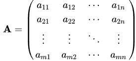
Algebraically, if A is an m x n matrix and B is an n x p matrix,
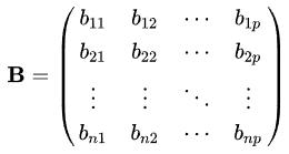
then the matrix product C = AB is determined to be the m x p matrix
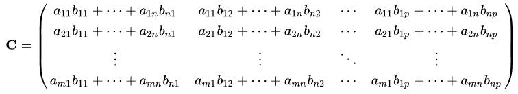
i.e.
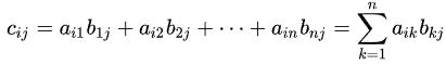
The Excel function MMULT returns the matrix product of two arrays, array1 and array2 (the Excel equivalent of a matrix). The result is an array with the same number of rows as array1 and the same number of columns as array2.
It has the following syntax:
MMULT(array1, array2)
where:
- array1 and array2 are required, and represent the two arrays you wish to multiply.
It should be noted that:
- as explained above, the number of columns in array1 must be the same as the number of rows in array2, and both arrays must contain only numbers
- array1 and array2 may be given as cell ranges, array constants or references
- MMULT returns the #VALUE! error when:
- any cells are empty or contain text
- the number of columns in array1 is different from the number of rows in array2
- The matrix product array, a, of two arrays, b and c, is:
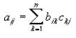
where i is the row number and j is the column number.
If you are using Microsoft 365, then you can simply enter the formula in the top left cell of the output range, then press ENTER to confirm the formula as a dynamic array formula. Otherwise, the formula must be entered as a legacy array formula by first selecting the output range, entering the formula in the top-left-cell of the output range, and then pressing CTRL + SHIFT + ENTER to confirm it. Excel inserts braces (curly brackets) automatically.
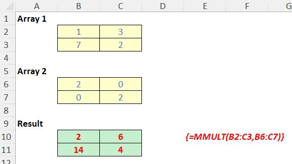
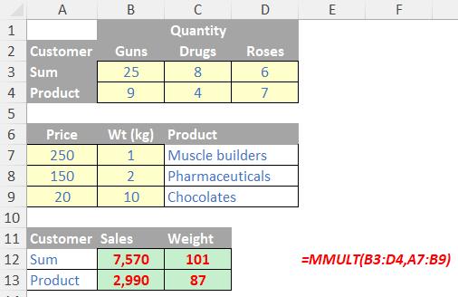
As examples:
Legacy Approach
Using Dynamic Arrays
We’ll continue our A to Z of Excel Functions soon. Keep checking back – there’s a new blog post every business day.
A full page of the function articles can be found here.