
Power Pivot Principles: Revisiting the SUM function
12 February 2019
Welcome back to our Power Pivot blog. Today, we discuss the SUM function.
It has just occurred to us that we have not formally covered the SUM function, despite using it in several other blogs: Measure Creation in Practice, Introducing Measures and Aggregations, and Variables in DAX, just to name a few.
In short, the SUM function adds all the numbers referenced. The syntax is very straightforward:
SUM(<reference>)
Example
As stated in our previous blogs, the SUM function serves as an aggregation function, which allows us to use it again in other measures such as CALCULATE. For example, we will receive an error if we were to type this measure into the DAX editor:
=CALCULATE(
'Sales Table'[Total Sales],
'Calendar'[Year]=2020
)
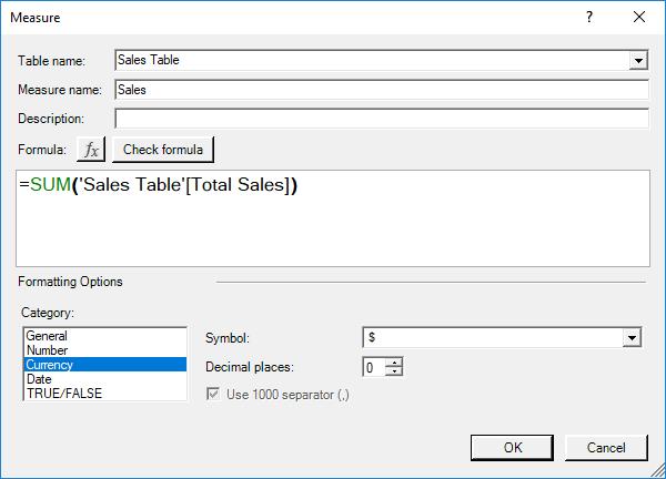
We have to create another measure with SUM to aggregate the column data before using it in our CALCULATE measure:
=SUM('Sales Table'[Total Sales])
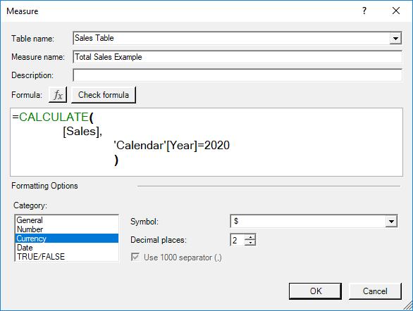
We can now insert the [Sales] measure that into our CALCULATE measure:
=CALCULATE(
[Sales],
'Calendar'[Year]=2020
)
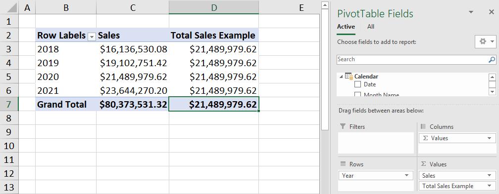
The resulting PivotTable would be as follows:
Shortfalls
The SUM function is great at aggregating or summing entire columns, however can it cope with summing the product of two columns at once? Consider the following data:
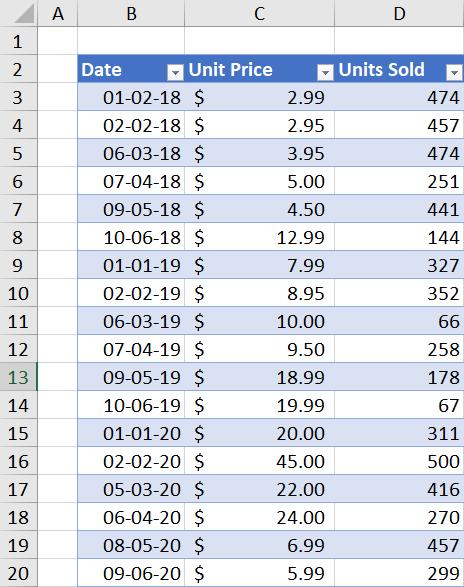
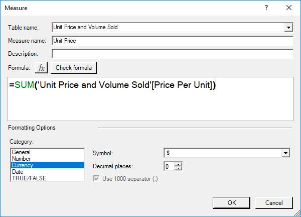
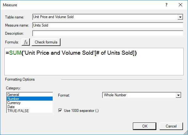
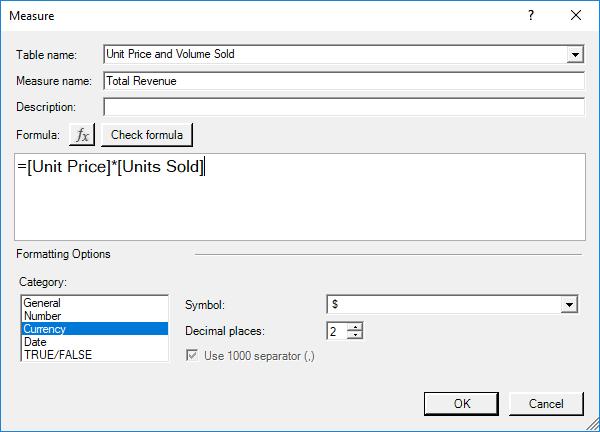
Let’s calculate the total revenue for our data. We will need to create three measures, [Unit Price], [Units Sold] and [Total Revenue]. These can be created as follows:
=SUM('Unit Price and Volume Sold'[Price Per Unit])
=SUM('Unit Price and Volume Sold'[# of Units Sold])
=[Unit Price]*[Units Sold]
The resulting PivotTable yields:
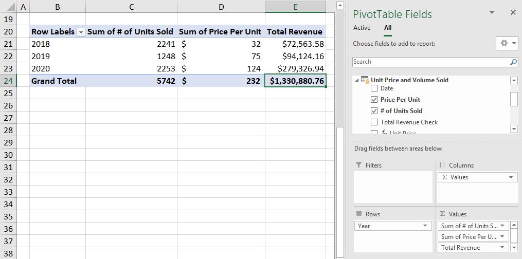
Strange, we didn’t think we made that much money either…
A quick and dirty check in our original data table reveals that we only made $72,678.89:
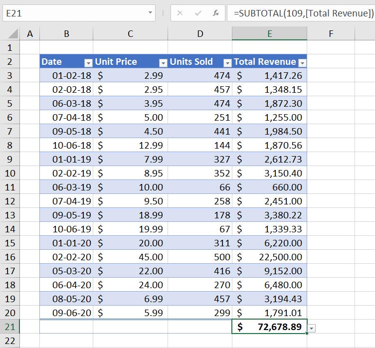
Upon further investigation it appears that the two columns are being aggregated first, then multiplied with each other to produce the total revenue (e.g. $32 * 2,241 = $72,563.58). The actual total revenue for 2018 should be $9,747.77.
How do we go about this? Well stay tuned, next week we will go over the SUMX function that solves this issue.
Until then, happy pivoting!
Stay tuned for our next post on Power Pivot in the Blog section. In the meantime, please remember we have training in Power Pivot which you can find out more about here. If you wish to catch up on past articles in the meantime, you can find all of our Past Power Pivot blogs here.