
A to Z of Excel Functions: The OFFSET Function
12 June 2023
Welcome back to our regular A to Z of Excel Functions blog. Today we look at the OFFSET function.
The OFFSET function
The older I get, the more invaluable OFFSET becomes. The syntax for OFFSET is as follows:
OFFSET(reference, rows, columns, [height], [width])
The arguments in square brackets (height and width) may be omitted from the function. The default values are the same dimensions as the original reference.
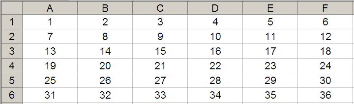
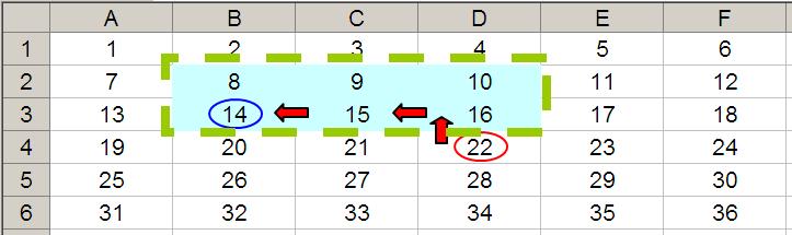
In its most basic form, OFFSET(ref, x, y) will select a reference x rows down (-x would be x rows up) and y columns to the right (-y would be y columns to the left) of the reference ref. For example, consider the following grid:
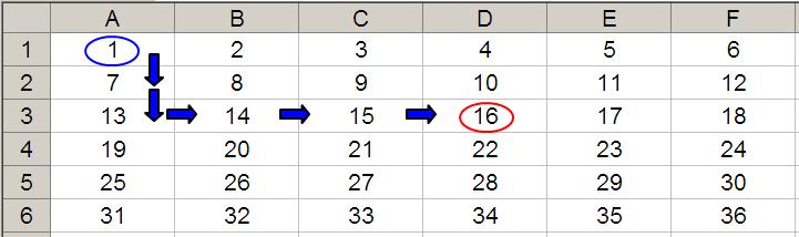
OFFSET(A1,2,3) would take us two rows down and three columns across to cell D3. Therefore, OFFSET(A1,2,3) = 16, viz.
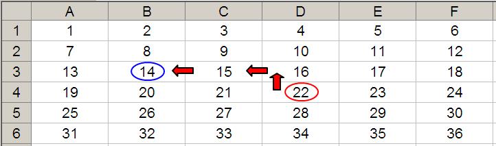
OFFSET(D4,-1,-2) would take us one row up and two rows to the left to cell B3. Therefore, OFFSET(D4,-1,-2) = 14, viz.
We can use these mechanics to construct a very simple scenario table:
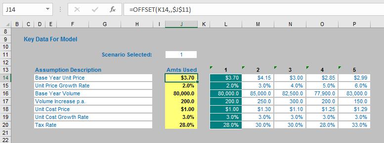
Essentially, the assumptions used in this illustration are linked from cells J14:J20 (in yellow). These values are drawn from the scenario table to the right of the highlighted yellow range (e.g. cells L14:L20 constitute Scenario 1, cells M14:M20 constitute Scenario 2).
The Scenario Selector is located in cell J11. Using OFFSET scenarios may be selected at will. For example, the formula in cell J14 is simply OFFSET(K14,,$J$11), that is, start at cell K14 and displace zero rows down and the value in J11 columns across. In the image above, the formula locates the cell one column to the right, which is Scenario 1.
The advantage of OFFSET over other functions such as INDEX, CHOOSE and LOOKUP functions is that the range of data can be added to. Whilst the other functions require a specified range whereas we can keep adding scenarios without changing the formula / making the model inefficient.
Furthermore, OFFSET can be used for other practical uses in Excel, taking advantage of the Height and Width arguments. Consider the OFFSET example from earlier. If we extend the formula to OFFSET(D4,-1,-2,-2,3), it would again take us to cell B3 but then we would select a range based on the Height and Width parameters. The Height would be two rows going up the sheet, with row 14 as the base (i.e. rows 13 and 14), and the Width would be three columns going from left to right, with column B as the base (i.e. columns B, C and D).
Hence OFFSET(D4,-1,-2,-2,3) would select the range B2:D3, viz.
Note that OFFSET(D4,-1,-2,-2,3) would result in a spilled array (or a #SPILL! error since Excel cannot display a matrix in one cell, but it does recognise it). Indeed, you may construct a simple depreciation calculation or transpose references using OFFSET’s Height and Width functionalities. But more on that another time…
There are a couple of problems with OFFSET.
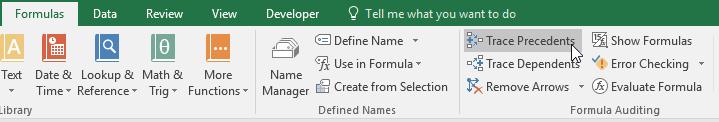
One of these problems is that values returned by an OFFSET function confuse Excel. Only the original reference is recognised as a precedent reference to the formula by Excel’s auditing tools.
The result returned is most likely to come from another cell which will not be highlighted by this technique. If you think about it, this actually makes sense as all of the cells on a worksheet are potential precedents.
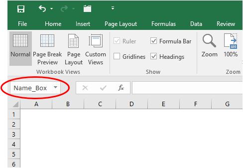
To take account of this, I suggest you give the reference a range name. by clicking on the cell and then typing the
desired name in the ‘Name box’
in Excel:
This range name should start with BC_. This prefix stands for “Base Cell” and makes it easier to sort / locate range names later. When users or model auditors alike inspect a formula with a Reference starting with BC_ for Base Cell (e.g. BC_Example_Reference), this can alert them to the fact that the model may be using cells in the region of this Reference that do not appear to have any dependents.
The other issue is that OFFSET is what is known as a volatile function. A volatile function is one that causes
recalculation of the formula in the cell where it resides every time Excel
recalculates. This can really slow down
your model if there are too many OFFSET functions, for example.
Aside: Volatile Functions
As stated above, a volatile function is one that causes recalculation of the formula in the cell where it resides every time Excel recalculates. This occurs regardless of whether precedent cells / calculations have changed, or whether the formula also contains non-volatile functions. One test to check whether your workbook is volatile is close a file after saving and see if Excel prompts you to save it a second time (this is an indicative test only). This can really slow down your model if there are too many OFFSET functions, for example.
Just because a function is volatile in one version of Excel does not mean it is volatile in all versions. Perhaps the best example of this is INDEX, which was volatile prior to Excel 97. Microsoft still states this function is volatile, but this does not appear to be the case except when used as the second part of a range reference, for example $A$1:INDEX($A$2:A$10,4), will also cause the reference to be flagged as “dirty” (i.e. needs to be recalculated) when the workbook is opened only.
Another common ‘semi-volatile’ function is SUMIF, which has been so since Excel 2002. This function becomes volatile whenever the size of the first range argument is not the same as the second (sum_range) argument, e.g. SUMIF(A1:A4,1,B1) is volatile whereas SUMIF(A1:A4,1,B1:B4) is not.
IF and CHOOSE do not calculate all arguments, but if any of the arguments are volatile – regardless of whether they are used – the formula is deemed to be volatile. Therefore, IF(1>0,1,RAND()) is always volatile, even though the value_if_false argument will never be calculated. It is not quite as simple as this though. If the formula in cell A1 is =NOW() then this cell will be volatile, but IF(1>0,1,A1) will not be.
In essence, direct references or dependents
of volatile functions will always be recalculated, whereas indirect ones will
only recalculate when activated or in certain other functions that always
calculate all arguments such as AND and OR.
We’ll continue our A to Z of Excel Functions soon. Keep checking back – there’s a new blog post every business day.
A full page of the function articles can be found here.