XLOOKUP and XMATCH: Two New X-Men for Excel

Late August 2019 and Microsoft has added two new functions, XLOOKUP and XMATCH. For reasons that will become clear, here I will mainly consider the former function – because once you understand XLOOKUP, XMATCH becomes obvious (nothing personal, XMATCH).

Therefore, let’s take a look at the new addition to the LOOKUP family. I so wanted it to be called FLOOKUP but it was not to be…

Ask anyone and they will tell you two “truths”:

1. They are a better than average driver and everyone else is an idiot on the roads
2. They are a better than average Excel user because they know how to use VLOOKUP.

It’s well known I hate VLOOKUP with a passion and if anything can come along and hurry its demise, well, I shall welcome it with open arms. Ladies and gentlemen, may I present the future of looking up for the masses – XLOOKUP. Hopefully, it will make an “ex” of VLOOKUP!

Why I Loathe VLOOKUP

Just as a recap, let me just summarise the resident incumbent:

has the following syntax:

• lookup_value: what value do you want to look up?
• table_array: where is the lookup table?
• column_index_number: which column has the value you want returned?
• [range_lookup]: do you want an exact or an approximate match?  This is optional and to begin with, I am going to ignore this argument exists.

HLOOKUP is similar, but works on a row, rather than a column, basis.

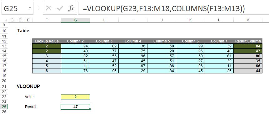
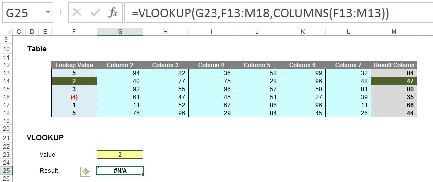
To show my disdain, I am going to use VLOOKUP throughout to keep things simple.  VLOOKUP always looks for the lookup_value in the first column of a table (the table_array) and then returns a corresponding value so many columns to the right, determined by the column_index_number.

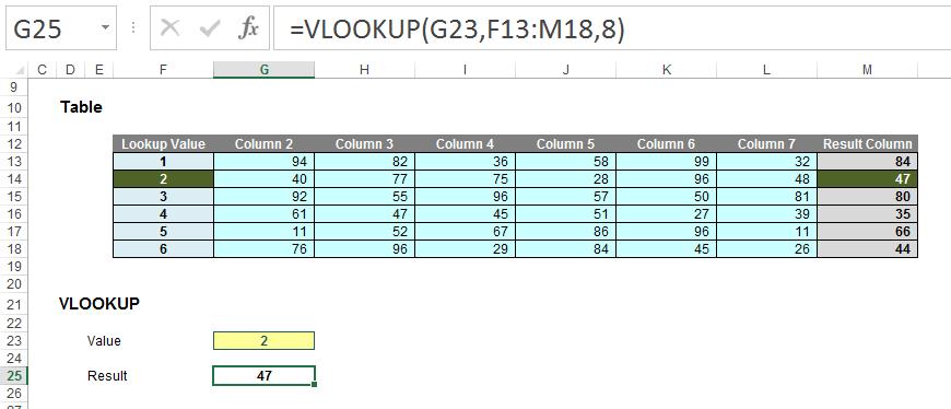
In this above example, the formula in cell G25 seeks the value 2 in the first column of the table F13:M18 and returns the corresponding value from the eighth column of the table (returning 47). 

Pretty easy to understand; so far so good.  So what goes wrong?  Well, what happens if you add or remove a column from the table range?

Adding (inserting) a column gives us the wrong value:

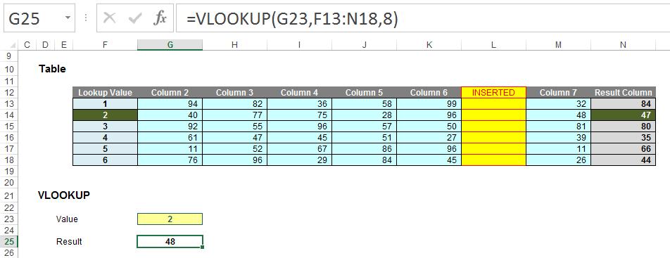
With a column inserted, the formula contain hard code (8) and therefore, the eighth column (M) is still referenced, giving rise to the wrong value. Deleting a column instead is even worse:

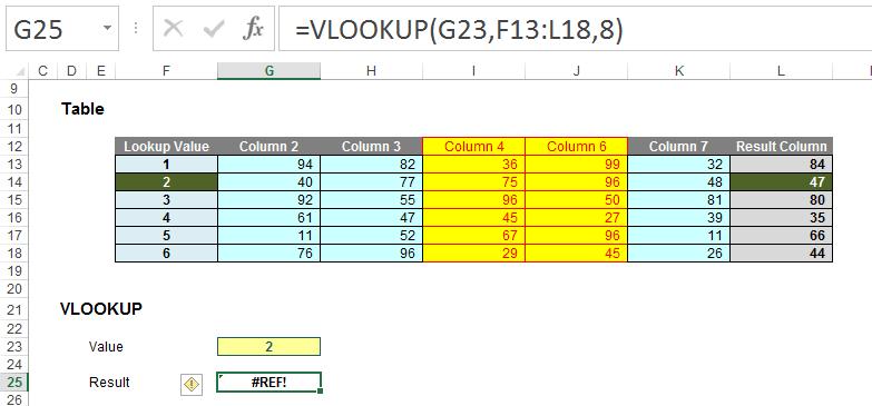
Now there are only seven columns so the formula returns #REF!  Oops.

It is possible to make the column index number dynamic using the COLUMNS function:

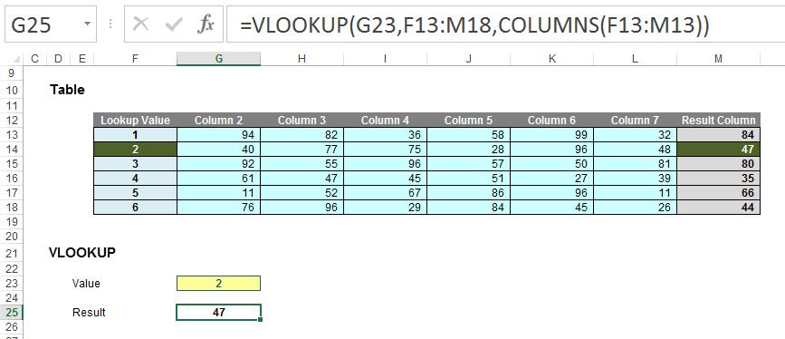
COLUMNS(reference) counts the number of columns in the reference.  Using the range F13:M13, this formula will now keep track of how many columns there are between the lookup column (F) and the result column (M).  This will prevent the problems illustrated above.

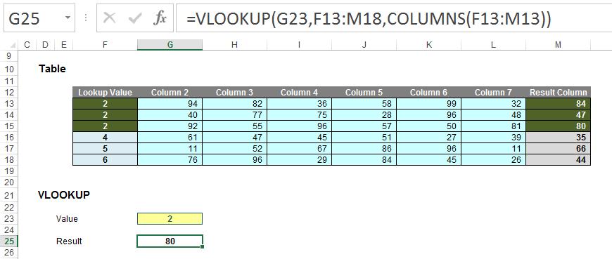
But there’s more issues.  Consider duplicate values in the lookup column.  With one duplicate, the following happens:

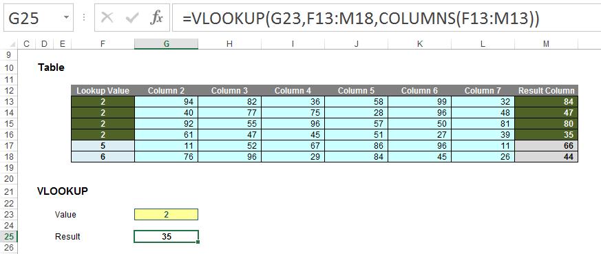
Here, the second value is returned, which might not be what is wanted. With two duplicates:

Ah, it looks like it might take the last occurrence. Testing this hypothesis with three duplicates:

Yes, there seems to be a pattern: VLOOKUP takes the last occurrence. Better make sure:

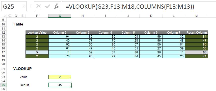
Rats. In this example, the value returned is the fourth of five. The problem is, there’s no consistent logic and the formula and its result cannot be relied upon. It gets worse if we exclude duplicates but mix up the lookup column a little:

In this instance, VLOOKUP cannot even find the value 2!

So what’s going on? The problem – and common modelling mistake – is that the fourth argument has been ignored:

[range_lookup] appears in square brackets, which means it is optional.  It has two values:

• TRUE: this is the default setting if the argument is not specified.  Here, VLOOKUP will seek an approximate match, looking for the largest value less than or equal to the value sought.  There is a price to be paid though: the values in the first column (or row for HLOOKUP) must be in strict ascending order – this means that each value must be larger than the value before, so no duplicates. 
  
  This is useful when looking up postage rates for example where prices are given in categories of pounds and you have 2.7lb to post (say).  It’s worth noting though that this isn’t the most common lookup when modelling.

• FALSE: this has to be specified.  In this case, data can be any which way – including duplicates – and the result will be based upon the first occurrence of the value sought.  If an exact match cannot be found, VLOOKUP will return the value #N/A.

And this is the problem highlighted by the above examples.  The final argument was never specified so the lookup column data has to be in strict ascending order – and this premiss was continually breached.

The robust formula needs both COLUMNS and a fourth argument of FALSE to work as expected:

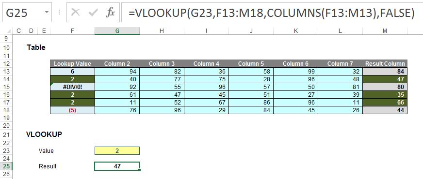
This is a very common mistake in modelling. Using a fourth argument of FALSE, VLOOKUP will return the corresponding result for the first occurrence of the lookup_value, regardless of number of duplicates, errors or series order. If an approximate match is required, the data must be in strict ascending order.

VLOOKUP (and consequently HLOOKUP) are not the simple, easy to use functions people think they are. In fact, they can never be used to return data for columns to the left (VLOOKUP) or rows above (HLOOKUP). So what should modellers use instead..?

Introducing XLOOKUP

There’s a new boss in town, but it’s only in selected towns presently. This function has been released in what Microsoft refers to as “Preview” mode, i.e. it’s not yet “Generally Available” but it is something you can try and hunt out. Presently, just like >dynamic arrays, you need to be part of what is called the “Office Insider” programme which is an Office 365 fast track. You can register in File -> Account -> Office Insider in Excel’s backstage area.

Even then, you’re not guaranteed a ticket to the ball as only some will receive the new function as Microsoft slowly roll out these features and functions.  Please don’t let that put you off.  This feature will be with all Office 365 subscribers soon.

XLOOKUP has the following syntax:

On first glance, it looks like it has too many arguments, but often you will only use the first three:

• lookup_value: this is required and defines what value you want to look up
• lookup_vector: this reference is required and is the row or column of data you are referencing to look up lookup_value
• results_array: this is where the corresponding item is you wish to return and is also required (even if it is the same as lookup_vector).  This does not have to be a vector (i.e. one row or one column of cells): it may be an array (with at least two rows and at least two columns of cells).  The only stipulation is that the number of rows / columns must equal the number of rows / columns in the column / row vector – but more on that later
• match_mode: this argument is optional.  There are four choices:
  • 0: exact match (default)
  • -1: exact match or else the largest value less than or equal to lookup_value
  • 1: exact match or else smallest value greater than or equal to lookup_value
  • 2: wildcard match.  You should use the special character ? to match any character and * to match any run of characters.
  What’s impressive, though, is that for certain selections of the final argument (search_mode), you don’t need to put your data in alphanumerical order!  As far as I am aware, this is a first for Excel
• search_mode: this argument is also optional.  There are again four choices:
  • 1: search first to last (default)
  • -1: search last to first
  • 2: what is known as a binary search, first to last (requires lookup_vector to be sorted).  Just so you know, a binary search is a search algorithm that finds the position of a target value within a sorted array.  A binary search compares the target value to the middle element of the array.  If they are not equal, the half in which the target cannot lie is eliminated and the search continues on the remaining half, again taking the middle element to compare to the target value, and repeating this until the target value is found
  • -2: another binary search, this time last to first (and again, this requires lookup_vector to be sorted).

XLOOKUP compares favourably with VLOOKUP

While VLOOKUP is the third most used function in Excel (behind SUM and AVERAGE), it has several well-known limitations which XLOOKUP overcomes: 

• it defaults to an “approximate” match: most often, users want an exact match, but this is not VLOOKUP’s default behaviour.  To perform an exact match, you need to set the final argument to FALSE (as explained earlier).  If you forget (which is easy to do), you’ll probably get the wrong answer
• it does not support column insertions / deletions: VLOOKUP’s third argument is the column number you’d like returned.  Since this is a hard-coded number, if you insert or delete a column you need to increment or decrement the column number inside the VLOOKUP – hence the need for the COLUMNS function (and the corresponding ROWS function for HLOOKUP)
• it cannot look to the left: VLOOKUP always searches the first column, then returns a column to the right.  There is no way to return values from a column to the left, forcing users to rearrange their data
• it cannot search from the bottom: If you want to find the last occurrence, you need to reverse the order of your data
• it cannot search for next larger item: when performing an “approximate” match, only the item less than or equal to the searched item can be returned and only if correctly sorted
• references more cells than necessary: VLOOKUP’s second argument, table_array, needs to stretch from the lookup column to the results column.  As a result, it typically references more cells than it truly depends on.  This could result in unnecessary calculations, reducing the performance of your spreadsheets.

Let’s have a look at XLOOKUP versus VLOOKUP:

You can clearly see the XLOOKUP function is shorter:

Only the first three arguments are needed, whereas VLOOKUP requires both a fourth argument, and, for full flexibility, the COLUMNS function as well.  XLOOKUP will automatically update if rows / columns are inserted or deleted.  It’s just simpler.

HLOOKUP has similar issues:

Here, this highlights what happens if I try to deduce the student name from the Student ID. HLOOKUP cannot refer to earlier rows, just as VLOOKUP cannot consider columns to the left. Given any unused elements of the table are ignored also, it’s just good news all round. Goodbye limitations, hello XLOOKUP.

Indeed, things get even more interesting when you start considering XLOOKUP’s final two arguments, namely match_mode and search_mode, viz.

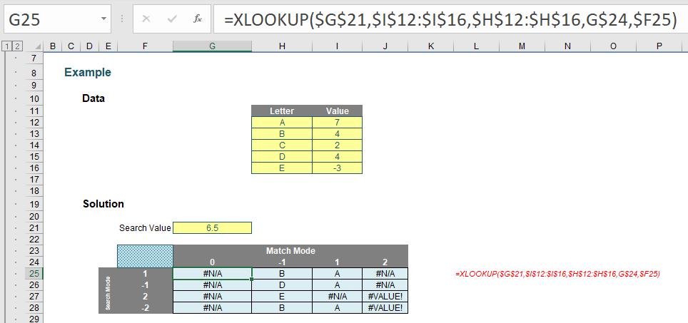
Notice that I am searching the ‘Value’ column, which is neither sorted nor contains unique items. However, I can look for approximate matches – impossible with VLOOKUP and / or HLOOKUP.

Do you see how the results vary depending upon match_mode and search_mode?

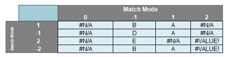
The match_mode zero (0) returns #N/A because there is no exact match.

When match_mode is -1, XLOOKUP seeks an exact match or else the largest value less than or equal to lookup_value (6.5). That would be 4 – but this occurs more than once (B and D both have a value of 4). XLOOKUP chooses depending upon whether it is searching top down (search_mode 1, where B will be identified first) or bottom up (search_mode -1, where D will be identified first). Note that with binary searches (with a search_mode of 2 or -2), the data needs to be sorted. It isn’t – hence we have garbage answers that cannot be relied upon.

With match_mode 1, the result is clearer cut. Only one value is the smallest value greater than or equal to 6.5. That is 7, and is related to A. Again, binary search results should be ignored.

The match_mode 2 results are spurious. This is seeking wildcard matches, but there are no matches, hence N/A for the only search_modes that may be seen as creditable (1 and -1).

Clearly binary searches are higher maintenance. In the past, it was worth investing in them as they did return results more quickly. However, according to Microsoft, this is no longer the case: apparently, there is “…no significant benefit to using (sic) the binary search options…”. If this is indeed the case, then I would strongly recommend not using them going forward with XLOOKUP.

To show how simple it now is to search from the end, consider the following:

This used to be an awkward calculation – but not anymore!  The formula is easy:

It’s a “standard” XLOOKUP formula, with a “bottom up” search coerced by using the final value of -1 (forcing the search_mode to go into “reverse”).

Comparisons with LOOKUP

Whilst XLOOKUP wins hands down against HLOOKUP and VLOOKUP, the same cannot necessarily be said for LOOKUP.  You may recall LOOKUP has two forms: an array form and a vector form.  As a reminder:

• an array is a collection of cells consisting of at least two rows and at least two columns
• a vector is a collection of cells across just one row (row vector) or down just one column (column vector).

The diagram should be self-explanatory:

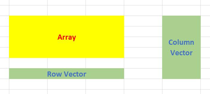
The array form of LOOKUP looks in the first row or column of an array for the specified value and returns a value from the same position in the last row or column of the same array:

where:

• lookup_value is the value that LOOKUP searches for in an array.  The lookup_value argument can be a number, text, a logical value, or a name or reference that refers to a value
• array is the range of cells that contains text, numbers, or logical values that you want to compare with lookup_value.

The array form of LOOKUP is very similar to the HLOOKUP and VLOOKUP functions.  The difference is that HLOOKUP searches for the value of lookup_value in the first row, VLOOKUP searches in the first column, and LOOKUP searches according to the dimensions of array.

If array covers an area that is wider than it is tall (i.e. it has more columns than rows), LOOKUP searches for the value of lookup_value in the first row and returns the result from the last row.  Otherwise, LOOKUP searches for the value of lookup_value in the first column and returns the result from the last column instead.

The alternative form is the vector form:

The LOOKUP function vector form syntax has the following arguments:

• lookup_value is the value that LOOKUP searches for in the first vector
• lookup_vector is the range that contains only one row or one column
• [result_vector] is optional – if ignored, lookup_vector is used – this is the where the result will come from and must contain the same number of cells as the lookup_vector.

Like the default versions of HLOOKUP and VLOOKUP, lookup_value must be located in a range of ascending values.

Let me demonstrate with an example:

LOOKUP is a great function to use with time series analysis / forecasting.  Dates are in ascending order and the LOOKUP syntax is remarkably simple.  As a modeller, I use it regularly when I am modelling many more forecast periods than I want assumption periods.

Here, you can see I carry assumptions only for 2020 until 2024 (the final value is 2024, just with a “+” in number formatting).  The formula

returns the corresponding value for the period that is either an exact match or else the largest value less than or equal to the lookup_value.  LOOKUP uses the top row of the table for looking up its data and the final row for returning the corresponding value.  Simple.  As for XLOOKUP:

This formula is longer and requires two additional arguments (match_mode -1 is required to mirror the behaviour of LOOKUP).  Indeed, given that an IF statement is required to ensure no errors for earlier periods, e.g.

it may be argued that LOOKUP is a simpler function to use here than its counterpart. 

This isn’t the only time LOOKUP outperforms XLOOKUP:

Here, we do see a limitation of XLOOKUP.  Whilst the third argument of XLOOKUP, results_array, does not need to be a vector, it cannot be the transposition of the lookup_vector.  You would have to transpose it using the TRANSPOSE function, for example.  This makes LOOKUP much easier to use – compare:

with

In this instance, LOOKUP wins.

Useful Features of XLOOKUP

XLOOKUP can be used to perform a two-way match, similar to >INDEX MATCH MATCH:

Many advanced users might use the formula

where:

• INDEX(array,  row_number, [column_number]) returns a value or the reference to a value from within a table or range (list) citing the row_number and the column_number
• MATCH(lookup_value, lookup_vector, [match_type]) returns the relative position of an item in an array that (approximately) matches a specified value.  It’s most commonly used with match_type zero (0), which requires an exact match.

Therefore, this formula finds the position in the row for the student and the position in the column of the subject.  The intersection of these two provides the required result.

XLOOKUP does it differently:

Welcome to the wonderful world of the nested XLOOKUP function!  Here, the internal formula

demonstrates a key difference between this and your typical lookup function – the first argument is a cell, the second argument is a column vector and the third is an array – with, most importantly, the same number of rows as the lookup_vector.  This means it returns a column vector of data, not a single value.  This is great news in the brave new world of dynamic arrays.

In essence, this means the formula resolves to

as J40:J46 is the resultant vector of =XLOOKUP(G51,H39:N39,H40:N46).  This is a really powerful – and virtually new – concept to get your head around, that admittedly SUMPRODUCT exploits too.  Once you understand this, it’s clear how this formula works and opens your eyes to the power of nested XLOOKUP functions.

I can’t believe I am talking about the virtues of nested functions here!  Let me change the subject quickly…

To show you how dynamic arrays can make the most of being able to create resultant vectors, consider the following example:

The formula

again resolves to a vector – but this time is allowed to spill as a dynamic array.  Obviously, this will only work in Office 365, but it’s a very useful tool that might just make you think it’s time to drop that perpetual licence.

Once you start playing with the dynamic range side, you can start to get imaginative.  For example:

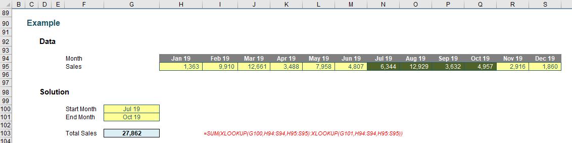
In this illustration, I want to calculate the sales between two periods:

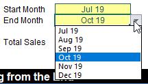
This might seem like a simple drop-down list using data validation (ALT + D + L), but XLOOKUP has been used in determining the list to be used for the end months.

Let me explain. I have hidden the range of relevant dates in cell H101 spilled across

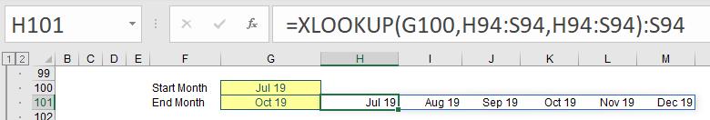
XLOOKUP can return a reference, so the formula

evaluates to the row vector N94:S94 (since the start month is July). This spilled dynamic array formula is then referenced in the data validation:

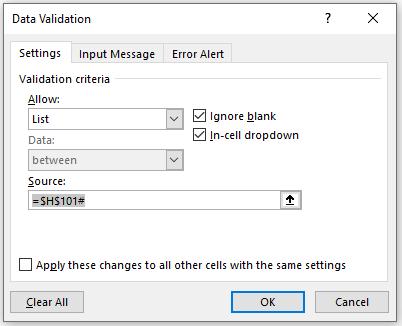
(You may recall $H$101# means the spilled range starting in cell H101.)  It should be noted that the formula =XLOOKUP(G100,H94:S94,H94:s94):S94 may not be used directly in the ‘Data Validation’ dialog, but this is a neat trick to ensure you cannot select an end month before the start month (assuming you are a rational human being that selects the start before the end!).

The formula to sum the sales then is

Again, this uses the fact XLOOKUP can return a reference, so this formula equates to

Easy!  Now I am combining two XLOOKUP formulae with a colon (:) to form a range.  This joins other illustrious functions used this way such as CHOOSE, IF, IFS, >INDEX, INDIRECT, OFFSET, >SINGLE (@), SWITCH and TEXT.  First nesting, now joining – what’s next?

Partial and Exact Matching

Seeking partial matches (sounds like an unfussy dating agency!) suddenly became a lot easier too. You can use wildcards if you want to – just set the match_mode to 2:

Here, I am searching for J?n*n* - which is fine as long as you know what the wildcard characters mean:

• ? means “any character”, but just one character.  If you wanted to make space for two and only two characters you would use ??
• * means “any number of characters’ – including zero.

For example, M?n*m* would identify “Manmade”, “minimum” and “Manikum” but would not accept “millennium”.  Here, our formulae

would locate the first and last items that satisfied the condition J?n*n* (i.e. “Jonathan” and “Jonny” respectively).

But what if you wanted an exact match with case sensitivity?  You just have to think a little but outside of the proverbial box:

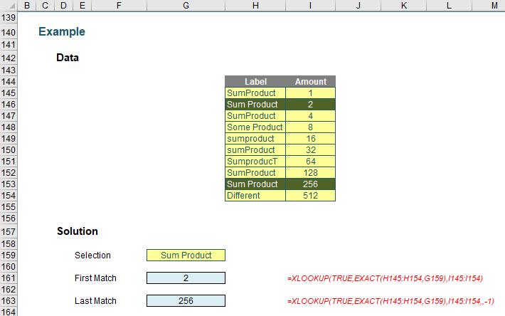
Here, we use another feature of XLOOKUP – its ability to search a virtual vector, i.e. one that has been constructed in memory, rather than physically within the spreadsheet cells.  Consider the formula

Here, the interim calculation =EXACT(H145:H154,G159), looks at the range H145:H154 and deduces whether the cells are an exact match for the selection ‘Sum Product’ in cell G159.  The EXACT function would evaluate as

{FALSE; TRUE; FALSE; FALSE; FALSE; FALSE; FALSE; FALSE; TRUE; FALSE}

Therefore, the formula coerces to

and then the formula becomes simple to understand.

No doubt there are many more great things you can do with XLOOKUP, but hey, it’s just arrived and we are only getting started!

XMATCH

As I said at the beginning, XLOOKUP did not land in isolation.  In addition to XLOOKUP, XMATCH has arrived with a similar signature to XLOOKUP, but instead it returns the index (position) of the matching item.  XMATCH is both easier to use and more capable than its predecessor MATCH.

XMATCH has the following syntax:

where:

• lookup_value: this is required and defines what value you want to look up
• lookup_vector: this reference is required and is the row or column of data you are referencing to look up lookup_value
• match_mode: this argument is optional.  There are four choices:
  • 0: exact match (default)
  • -1: exact match or else the largest value less than or equal to lookup_value
  • 1: exact match or else smallest value greater than or equal to lookup_value
  • 2: wildcard match.  You should use the special character ? to match any character and * to match any run of characters.
  Again, for certain selections of the final argument (search_mode), you don’t need to put your data in alphanumerical orderain, for certain selections of the final argument (
• search_mode: this argument is also optional.  There are again four choices:
  • 1: search first to last (default)
  • -1: search last to first
  • 2: this is a binary search, first to last (requires lookup_vector to be sorted)
  • -2: another binary search, this time last to first (and again, this requires lookup_vector to be sorted).

As you can see, it’s a fairly straightforward addition to the MATCH family.  It acts similarly to MATCH – just with heaps more functionality.

Word to the Wise

XLOOKUP and XMATCH open up new avenues for Excel to explore, but it must be remembered they are still in Preview and may only be accessed by a lucky few on the Insider track.  Feel free to download and play with the attached Excel file, but don’t be too perturbed if your version of Excel does not recognise these functions yet.