
Spreadsheet Skills: New Excel 2016 Functions and Features
This month we take a break from reader’s questions to bring you a newsflash: Excel 2016 has released a half dozen new functions – but not every 2016 user will be getting them...
By Liam Bastick, Managing Director (and Excel MVP) with SumProduct Pty Ltd.
Introduction
Most of the time I write articles that do not matter whether you, dear reader, are using Excel 2016, Excel 97 or an abacus (OK, so I might be exaggerating slightly). However, more and more users are migrating to the Office 365 subscription model and with that comes great power, well Excel 2016 anyway. And some versions of Office 365 Excel 2016 are getting six new functions to play with. The roll-out started in late February – too late for me to report in last month’s article – but I thought it would be well worth reviewing these new entrants to the Excel family.
Do note I said some Excel users are getting these new features. To have access to these functions, you have to meet one of the following requirements:
- You are an Office 365 subscriber and have the latest version of Office installed on your PC
- You are using Excel Online
- You are using Excel Mobile
- You are using Excel for Android phones and tablets.
Just having standalone Office 2016 is insufficient: Microsoft’s push to get everyone onto the subscription model continues! Even then, the roll-out will be in stages. Office 365, Home, Personal or University subscriptions will update before other types and businesses may find new features have been restricted by their IT departments. Further, recent discussions on Excel for a suggest PCs may be getting new features ahead of those with Mac’s etc.
There are six new Excel functions in Excel 2016 Remixed. I will now look at each one in turn.
IFS
As a model developer and reviewer, I must confess I am not convinced about this one. If you have ever used a formula with nested IF statements, e.g. =IF(IF(IF…
then maybe this function is for you – however, if you have ever written Excel formulae like this, then maybe Excel isn’t for you! There are usually better ways of writing the formula using CHOOSE or INDEX(MATCH) (see the >INDEX MATCH article) for example.
The syntax is as follows:
IFS(logical_test1, value_if_true1, [logical_test2, value_if_true2], [logical_test3, value_if_true3],…)
where:
- logical_test1 is a logical condition that evaluates to TRUE or FALSE;
- value_if_true1 is the result to be returned if logical_test1 evaluates to TRUE. This may be empty
- logical_test2 (and onwards) are further conditions that evaluate to TRUE or FALSE also
- value_if_true2 (and onwards) are the respective results to be returned if the corresponding logical_test evaluates to TRUE. Any or all may be empty.
Since functions are limited to 254 arguments (sometimes known as parameters), the new IFS function can contain 127 pairs of conditions and results.
One thing to note is that IFS is not quite the same as IF. With the IF statement, the third argument corresponds to what do if the logical_test is not TRUE (i.e. it is an ELSE condition). IFS does not have an inherent ELSE condition, but it can be easily generated. All you have to do is make the final logical_test equal to a condition which is always trues such as TRUE or 1=1 (say).
Other issues to consider:
- Whilst the value_if_true may be empty, it must not be omitted. Having an odd number of arguments in an IFS statement would give rise to the “You’ve entered too few arguments for this function” error message.
- If a logical_test is not actually a logical test (e.g. it evaluates to something other than TRUE or FALSE, the function returns an #VALUE! error. Numbers still appear to work though: any number than zero evaluates as TRUE and zero is considered to be FALSE.
- If no TRUE conditions are found, this function returns the #N/A! error.
To show how it works, consider the following example.
IFS Example
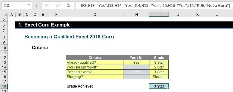
Here, would-be gurus are graded based on evaluation criteria in the table, applied in a particular order:
=IFS(H13="Yes",I13,H14="Yes",I14,H15="Yes",I15,H16="Yes",I16,TRUE,"Not a Guru")
I think it’s safe that although it is reasonably straightforward to follow, it is entirely reasonable to say it’s not the prettiest, most elegant formula ever put to Excel paper. In particular, do pay heed to the final logical_test: TRUE. This ensures we have an ELSE condition as discussed above.
To be fair, one similar solution using legacy Excel functions isn’t any better:
=IF(H13="Yes",I13,IF(H14="Yes",I14,IF(H15="Yes",I15,IF(H16="Yes",I16,"Not a Guru"))))
Lovely.
This example (and another one using leap years) can be found in this month’s attached Excel file.
SWITCH
SWITCH is already available in many alternative programming languages and can simplify potentially horrible formulae. This function evaluates an expression against a list of values and returns the result corresponding to the first matching value. If there is no match, an optional default value may be returned. The syntax is as follows:
SWITCH(expression, value1, result1, [default or value2, result2],…[default or valueN, resultN])
where:
- expression is the value that will be compared against the values (value1 to valueN) cited
- value1 to valueN are the values that will be compared against the expression
- result1 to result are the values, references or formulae results to be returned when the corresponding valueN argument matches the expression. The result must be supplied for each corresponding valueN argument
- default is an optional value to return in case no matches are found in the valueN expressions. The default argument is identified by having no corresponding result expression, i.e. it must be the final argument in the function where the function contains an odd, rather than an even, number of arguments. If no default argument is supplied and no match is found this function returns the #N/A! error.
To illustrate, consider the following painful formula:
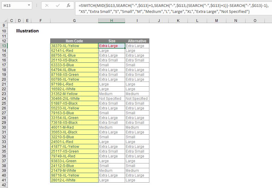
=SWITCH(MID($G13,SEARCH("-",$G13)+1,SEARCH("-",$G13,(SEARCH("-",$G13)+1))-SEARCH("-",$G13)-1),"XS","Extra Small","S","Small","M","Medium","L","Large","XL","Extra Large","Not Specified")
SWITCH Example
The expression here is
MID($G13,SEARCH("-",$G13)+1,SEARCH("-",$G13,(SEARCH("-",$G13)+1))-SEARCH("-",$G13)-1)
which is determining what is contained between the two hyphens (for more on text string functions, please see this article). It is horrible, and that’s the point. The formula then considers what the values may be (“XL”,”M”) and what value should be returned as a consequence (“Extra Large”, “Medium”).
The corresponding Excel formula before SWITCH would have been a nightmare:
=IF(MID($G13,SEARCH("-",$G13)+1,SEARCH("-",$G13,(SEARCH("-",$G13)+1))-SEARCH("-",$G13)-1)="XS","Extra Small",IF(MID($G13,SEARCH("-",$G13)+1,SEARCH("-",$G13,(SEARCH("-",$G13)+1))-SEARCH("-",$G13)-1)="S","Small",IF(MID($G13,SEARCH("-",$G13)+1,SEARCH("-",$G13,(SEARCH("-",$G13)+1))-SEARCH("-",$G13)-1)="M","Medium",IF(MID($G13,SEARCH("-",$G13)+1,SEARCH("-",$G13,(SEARCH("-",$G13)+1))-SEARCH("-",$G13)-1)="L","Large",IF(MID($G13,SEARCH("-",$G13)+1,SEARCH("-",$G13,(SEARCH("-",$G13)+1))-SEARCH("-",$G13)-1)="XL","Extra Large","Not Specified")))))
Both examples may be found in this month’s attached Excel file.
To be honest, I wouldn’t use either approach. I would have the expression in one cell and then use a lookup table to return the corresponding value for the result produced. But hey, that’s me.
CONCAT
This function replaces the CONCATENATE function. The CONCAT function combines the text from multiple ranges and / or text strings:
CONCAT(text1, [text2],…)
where:
- text1 is the text item to be joined
- text2 (onwards) are the additional items to be joined.
For example, consider the following illustration:
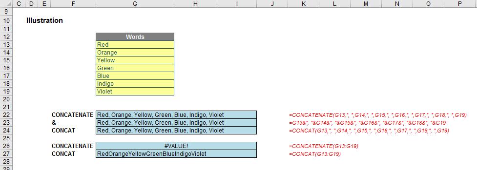
CONCAT Example
Upon first glance, CONCAT does the same thing as the legacy CONCATENATE function or & (ampersand) operator, but is just easier to spell. However, it is a little more than that: CONCATENATE will not cope with highlighting a contiguous range (it will just return the #VALUE! error); CONCAT will concatenate them all.
Again, these examples may be found in this month’s attached Excel file, but perhaps a better one to review there is the TEXTJOIN function instead…
TEXTJOIN
The TEXTJOIN function combines the text from multiple ranges and / or text strings and includes a delimiter to be specified between each text value to be combined. If the delimiter is an empty text string, this function will effectively concatenate the ranges similarly to the CONCAT function. Its syntax is
TEXTJOIN(delimiter, ignore_empty, text1, [text2], …)
where:
- delimiter is a text string (which may be empty) with characters contained within inverted commas (double quotes). If a number is supplied, it will be treated as text
- ignore_empty ignores empty cells if TRUE or the argument is unspecified (i.e. is blank)
- text1 is a text item to be joined
- text2 (onwards) are additional items to be joined up to a maximum of 252 arguments. If the resulting string contains more than 32,767 characters TEXTJOIN returns the #VALUE! error.
TEXTJOIN is more powerful than CONCAT. To highlight this, consider the following examples:
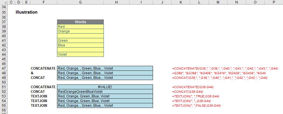
TEXTJOIN Example
Here, in the formulae on rows 53 and 54, empty cells in a contiguous range may be ignored and delimiters only need to be specified once. When you compare to CONCAT, you do begin to wonder why you need it – perhaps to soften the demise of CONCATENATE..?
MAXIFS and MINIFS
The last two new functions I am going to combine – and not with TEXTJOIN!
MAXIFS(max_range, criterion_range1, criterion1, [criterion_range2, criterion2], ...)
returns the maximum value among cells specified by a given set of conditions or criteria, where:
- max_range is the actual range of cells in which the maximum is to be determined
- criterion_range1 is the set of cells to evaluate with the criterion specified
- criterion1 is the criterion in the form of a number, expression or text that defines which cells will be evaluated as a maximum
- criterion_range2 (onwards) and criterion2 (onwards) are the additional ranges and their associated criteria. 126 range / criterion pairs may be specified. All ranges must have the same dimensions otherwise the function returns an #VALUE! error.
MINIFS behaves similarly but returns the minimum rather than the maximum value among cells specified by a given set of conditions or criteria.
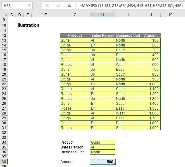
MAXIFS Example
This example and a similar MINIFS example may be found in the attached Excel file.
This example is preferable to its standard Excel counterpart:
{=MAX(IF(G13:G31=H34,IF(H13:H31=H35,IF(I13:I31=H36,J13:J31))))}
Array formulae (see this article for more information) are cumbersome and not readily understood.
Other Updates
The recent update didn’t end with the six new functions. Microsoft improved the AutoComplete functionality in that you no longer need to be so precise to find what you are looking for, e.g.
AutoComplete Example
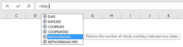
Excel will now look for functions or range names that contain the phrase sought. This will help immensely when you cannot quite remember what it was you are looking for.
A new chart type has been added too:
Funnel Charts Example
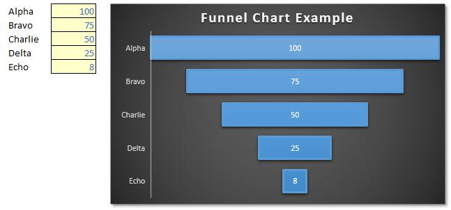
Funnel charts are a type of symmetrical bar chart. They were easy to construct before and slightly easier now. I don’t wish to sound churlish, but it’s not quite a waterfall chart!
And finally, something I think the majority of readers will possibly agree they may well be able to live without. Let me introduce you to Office 2016’s brand new Black theme:
New Black Office Theme
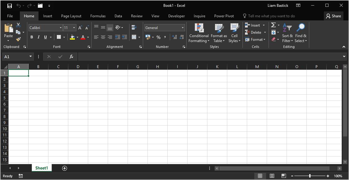
Perfect for hangovers and for reflecting your mood when you have to work late, I am not quite sure this is going to catch on. In fact, I am so convinced I am not even bothering explaining how to get it!!
Word to the Wise
Be careful if you decide to jump in head first and start using these new functions and features. Early adoption is not without its problems, as colleagues may not be able to use spreadsheets that take advantage of these new options. I would strongly recommend checking with your intended end users what version of Excel they have before building your first nested IFS function (and please, don’t do that…).
If you have a query for the Spreadsheet Skills section, please feel free to drop Liam a line at liam.bastick@sumproduct.com.