
Lookout for VLOOKUP and HLOOKUP
As a professional modeller, Liam Bastick highlights some of the common mistakes prevalent in financial modelling / Excel spreadsheeting. This article considers how to look out for V and H LOOKUP.
A Common Scenario
Often you will need to look up data in a table – and two functions most modellers are very familiar with are VLOOKUP and HLOOKUP. But do you realise it’s very easy to make a mistake with these functions?
Let’s start with a refresher.
VLOOKUP(lookup_Value,table_array,col_index_num,[range_lookup]) has the following syntax:
- lookup_value: What value do you want to look up?
- table_array: Where is the lookup table?
- col_index_num: Which column has the value you want returned?
- [range_lookup]: Do you want an exact or an approximate match? This is optional and to begin with, I am going to ignore this argument exists.
HLOOKUP is similar, but works on a row rather than a column basis.
Example
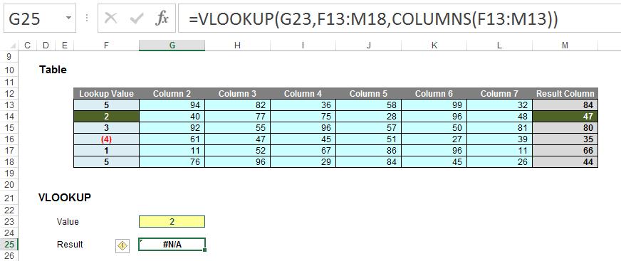
I am going to use VLOOKUP throughout to keep things simple. VLOOKUP always looks for the lookup_value in the first column of a table (the table_array) and then returns a corresponding value so many columns to the right, determined by the col_index_num column index number.
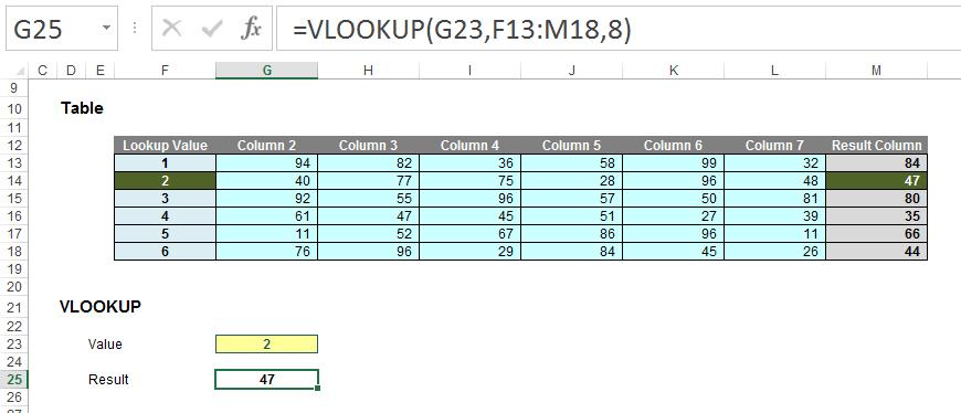
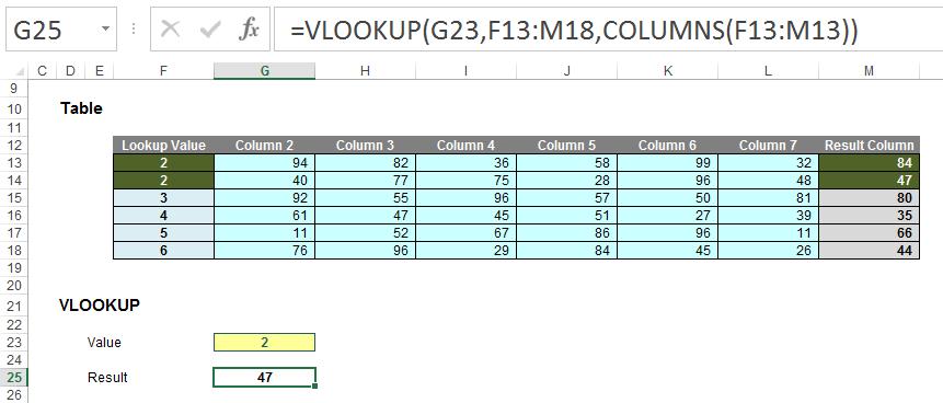
In this above example, the formula in cell G25 seeks the value 2 in the first column of the table F13:M18 and returns the corresponding value from the eighth column of the table (returning 47). You can follow all of these examples in the attached Excel file.
Pretty easy to understand – so far so good. So what goes wrong? Well, what happens if you add or remove a column from the table range?
Adding gives us the wrong value:
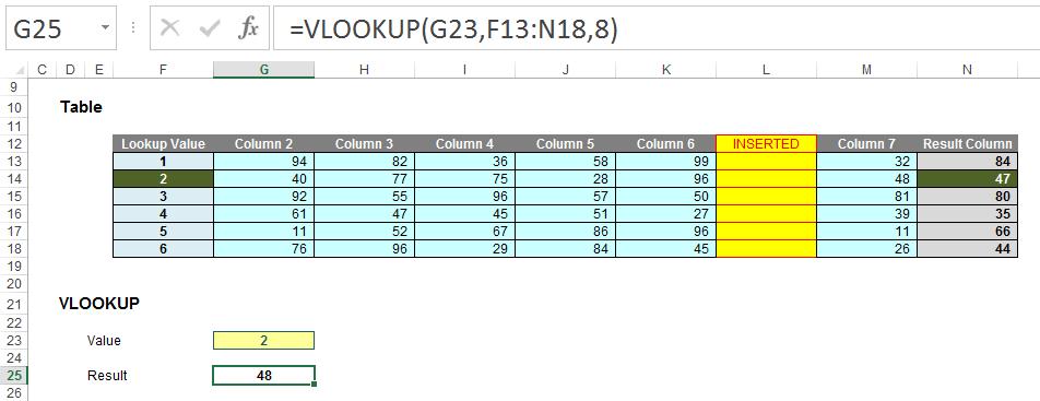
With a column inserted, the formula contain hard code (8) and therefore, the eighth column (M) is still referenced, giving rise to the wrong value.
Deleting a column instead is even worse:
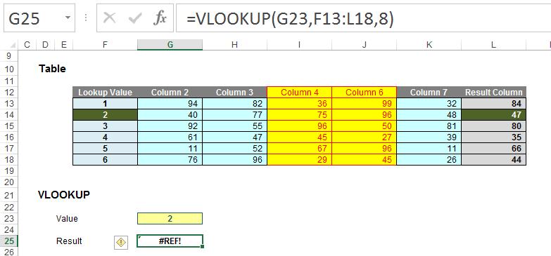
Now there are only seven columns so the formula returns #REF! Oops.
It is possible to make the column index number dynamic using the COLUMNS function:
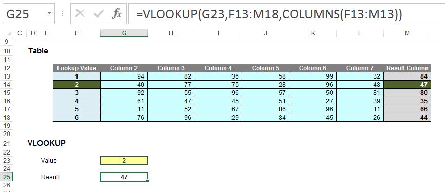
COLUMNS(reference) counts the number of columns in the reference. Using the range F13:M13, this formula will now keep track of how many columns there are between the lookup column (F) and the result column (M). This will prevent the problems illustrated above.
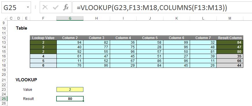
But there’s more issues. Consider duplicate values in the lookup column. With one duplicate, the following happens:
Here, the second value is returned, which might not be what is wanted. With two duplicates:
Ah, it looks like it might take the last occurrence. Testing this hypothesis with three duplicates:
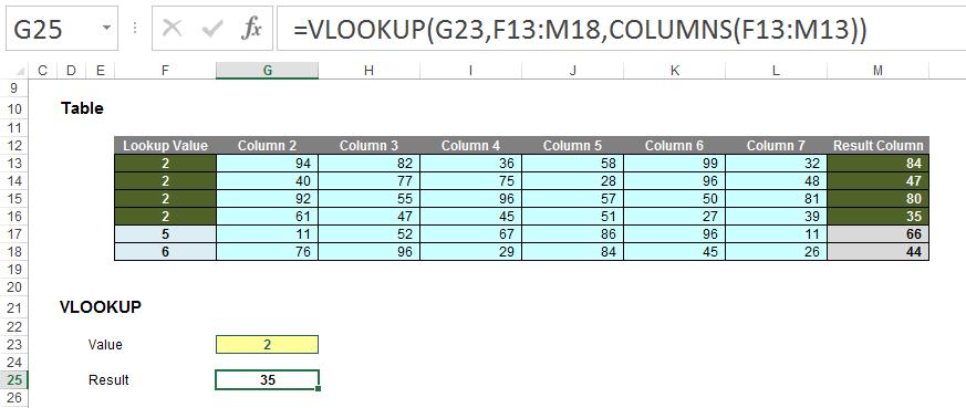
Yes, there seems to be a pattern: VLOOKUP takes the last occurrence. Better make sure:
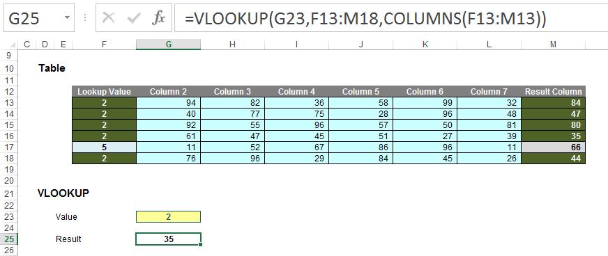
Rats. In this example, the value returned is the fourth of five. The problem is, there’s no consistent logic and the formula and its result cannot be relied upon. It gets worse if we exclude duplicates but mix up the lookup column a little:
In this instance, VLOOKUP cannot even find the value 2!
So what’s going on? The problem – and common modelling mistake – is that the fourth argument has been ignored:
VLOOKUP(lookup_Value,table_array,col_index_num,[range_lookup])
[range_lookup] appears in square brackets, which means it is optional. It has two values:
- TRUE: this is the default setting if the argument is not specified. Here, VLOOKUP will seek an approximate match, looking for the largest value less than or equal to the value sought. There is a price to be paid though: the values in the first column (or row for HLOOKUP) must be in strict ascending order – this means that each value must be larger than the value before, so no duplicates.
This is useful when looking up postage rates for example where prices are given in categories of kilograms and you have 2.7kg to post (say). It’s worth noting though that this isn’t the most common lookup when modelling.
- FALSE: this has to be specified. In this case, data can be any which way – including duplicates – and the result will be based upon the first occurrence of the value sought. If an exact match cannot be found, VLOOKUP will return the value #N/A.
And this is the problem highlighted by the above examples. The final argument was never specified so the lookup column data has to be in strict ascending order – and this premiss was continually breached.
The robust formula needs both COLUMNS and a fourth argument of FALSE to work as expected:
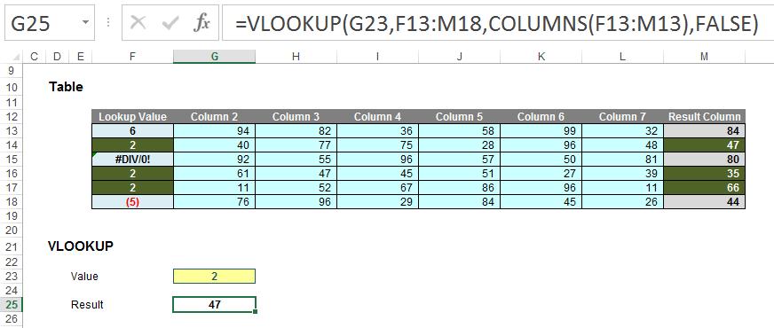
This is a very common mistake in modelling. Using a fourth argument of FALSE, VLOOKUP will return the corresponding result for the first occurrence of the lookup_value, regardless of number of duplicates, errors or series order. If an approximate match is required, the data must be in strict ascending order.
VLOOKUP (and consequently HLOOKUP) are not the simple, easy to use functions people think they are. In fact, they can never be used to return data for columns to the left (VLOOKUP) or rows above (HLOOKUP). So what should modellers use instead..?
Check out our articles on >INDEX and MATCH and Looking up to LOOKUP for more.
Word to the Wise
As stated above, HLOOKUP works like VLOOKUP but hunts out a value in the first row of a table and returns a value so many rows below this reference. However, it has the same limitations and should be used just as carefully.