Monday Morning Mulling: February 2022 Challenge

On the final Friday of each month, we set an Excel / Power Pivot / Power Query / Power BI problem for you to puzzle over for the weekend.  On the Monday, we publish a solution.  If you think there is an alternative answer, feel free to email us.  We’ll feel free to ignore you.

The challenge this month was to spill a range of cells that unpivot some last columns of an array.  Easy, yes?

The Challenge

Sometimes, when you work with pivoted data that has a structure similar to a PivotTable, it is difficult to look up a value based on multiple column and row criteria.  To make it simpler, we usually unpivot the data.  Most of the time, you may choose to use Unpivot Columns function in Power Query.

This challenge was designed to make you think outside the box to find another way using only Excel formulas.  You can download the question file here.

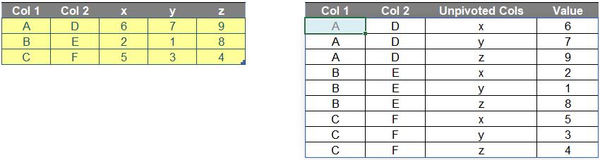
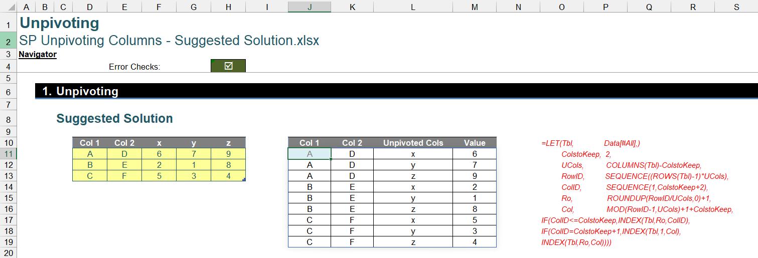
This month’s challenge was to write a formula in one cell using Dynamic Arrays that would spill a range of cells to unpivot only the last three [3] columns (i.e. x, y and z) of the array in the file above.  The result should look like the array generated on the right (below):

As always, there were some requirements:

• the formula needed to be in just one cell (no “helper” cells)
• this was a formula challenge; no Power Query / Get & Transform or VBA!
• the formula needed to be flexible, so that if we adjusted the number of rows and / or columns of the input table, the formula should still work
• obviously, the numbers of rows / columns of the output table could not exceed the row / column limitations of Excel.

Suggested Solution

You can find our Excel file here which demonstrates our suggested solution.  However, before explaining our solution, we will clarify how we came up with it first.

Brainstorming

Firstly, inputs of the formula include:

• Data table in the question
• number of columns that will not be unpivoted, which is two [2] (i.e. Col 1 and Col 2).  We name it as ColstoKeep.

Therefore, the number of columns to unpivot is three [3], which is calculated as below.  We name this number as UCols.

Secondly, we need to consider some features (e.g. numbers of rows and columns) of the output array.  After we unpivot the table, they should be calculated as below:

• Number of rows: 9

• Number of columns: 4.  The output table will include the first two [2] columns of initial table and two [2] additional columns for the old Row Headers (i.e. x, y and z) and Values (i.e. numbers in Data table in this case).

Thirdly, to create a Dynamic Range for the output, we need the help of INDEX and SEQUENCE.

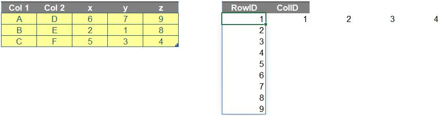
The row and column index numbers of output need to be created by SEQUENCE as follows.  We will call them RowID and ColID.

• RowID:

• ColID:

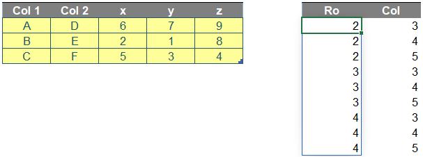
Additionally, we need to identify row and column positions of the Values in Data.  We will call them Ro and Col.

For example, number ‘7’ is located on row 2 and column 4 of Data.

• Ro:

• Col:

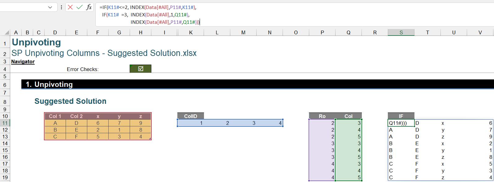
Finally, the trick of this challenge is to use ColID with an IF statement (below) as a connector for three different INDEX functions, i.e.

“If ColID is less than or equal to ColstoKeep, then get the first two [2] columns of Data,

else if ColID is equal to ColstoKeep + 1, then get the Row Header of unpivoted columns of Data,

else get the Values of Data.”

The result is as follows:

Returning to the Suggested Solution

You may wonder why the challenge only allows a formula cell when there are several working steps above.  Our solution is a combination of all described steps above within a LET formula as follows:

There are seven [7] variables:

• Tbl is an input table to unpivot
• ColstoKeep is the number of first columns you do not want to unpivot
• UCols is the number of unpivoted columns
• RowID and ColID are row and column indices of the output table
• Ro and Col are initial row and column positions of Values in the input table.

Then, the final part of the formula is the calculation to unpivot the last three [3] columns, viz.

Although it is a long and complex formula, you can apply it to your input table by only replacing the values of Tbl and ColstoKeep.

The Final Friday Fix will return on Friday 25 March 2022 with a new Excel Challenge.  In the meantime, please look out for the Daily Excel Tip on our home page and watch out for a new blog every business working day.