Charts and Dashboards: Dynamic Simulation Charts

Happy New Year!

Welcome back to this week’s Charts and Dashboards blog series. As the first blog of the year, we will create a dynamic simulation chart.

A while ago, on SumProduct’s Thought page, we discussed simulations, where we applied simulation analysis in Excel and created several charts, e.g.

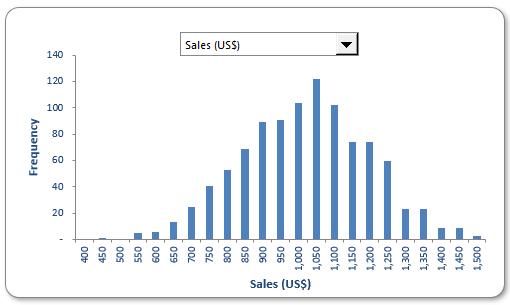
This time, we will go through the steps of creating one. The attached Excel file can be used in practice.

The above column chart has dynamic series and axes defined as ‘Chart_Stratification’ and ‘Chart_Count’, which change by the choice from the drop-down list. It only requires a quick collation step to summarise the outputs graphically.

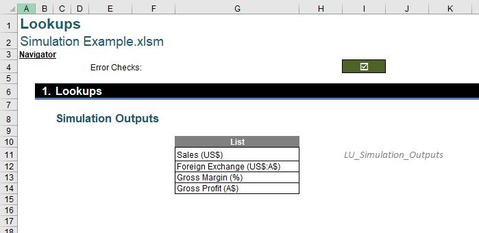
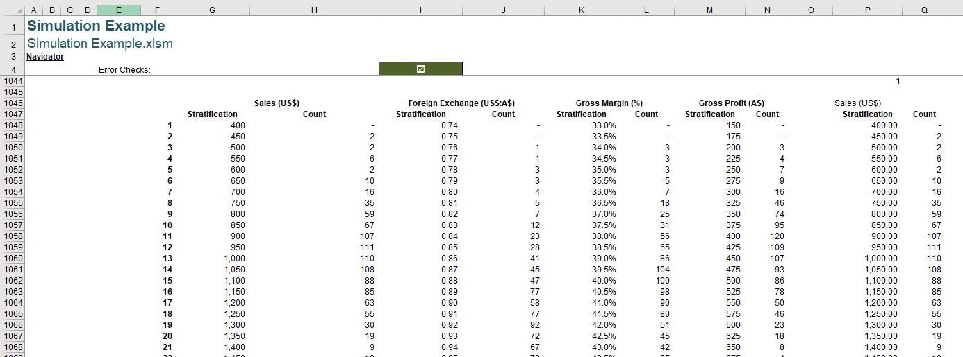
First, in the Lookups sheet, define the ‘LU_Simulation_Outputs’ range (cell G11:G14).

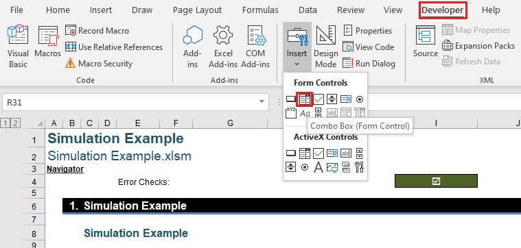
Now, to create the drop-down list, navigate to the Developer tab on the Ribbon, from Insert, choose ‘Combo Box (Form Control)’ and draw a drop-down list box.

Then, right-click on the drop-down list box and choose ‘Format Control’. Link the ‘Input range’ and ‘Cell link’. The number of ‘Drop down lines’ should be eight (8).

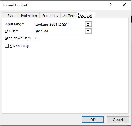
The cell P1044 is named ‘DD_Simulations_Outputs’, which is the indication of the drop-down choice.

The formula in cell P1046 is

The OFFSET function is used to get the Stratification and Count, respectively:

and

Next, define the dynamic range name using the OFFSET function:

Select the value in the Stratification and Count columns to create a Column chart, then right-click on the chart and choose ‘Select Data...’.

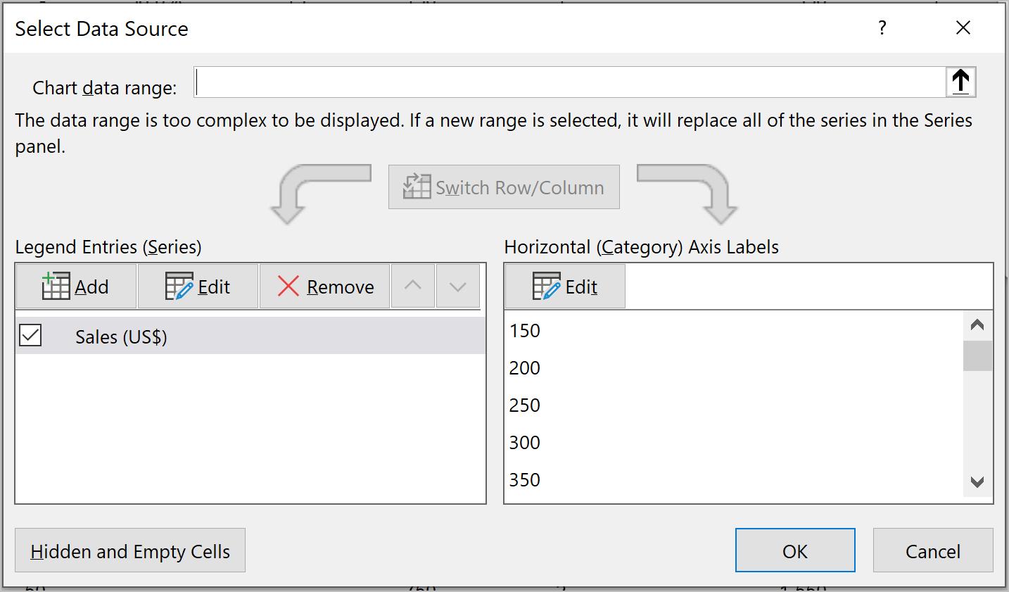
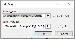
Let the ‘Series values’ take the dynamic ‘Chart_Count’ range

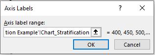
and ‘Axis label range’ be the ‘Chart_Stratification’ range. Please note that the sheet name should also be included.

Last but not least, make the axis label dynamic by point it to the cell 'Simulation Example'!$P$1046.

That’s it for this week. Check back next week for more Charts and Dashboards tips.