Simulation Stimulation

Risk and uncertainty are prevalent in all business decisions we make. Using simulations analysis, it is possible to quantify and analyse their impact. Here, we look at how to undertake simple simulations analysis using nothing more than Excel and some of its lesser known functions and functionalities. By Liam Bastick, director with SumProduct Pty Ltd.

Query

I use various “what-if?” analysis techniques within my spreadsheets such as scenario and sensitivity analysis. A colleague has suggested I undertake Monte Carlo simulations analysis too. Could you shed some light on what this is and how I could apply it in Excel?

Advice

I am fortunate enough to have presented at various technical conferences around the world and one thing I have noticed that always attracts delegates in their droves is the mention of “simulation(s) analysis”. However, before I explain the principles of this technique, it may be worthwhile to review the other approaches mentioned above:

• Scenario analysis is a common top-down analytical approach where numerous inputs are modified at a time, consistent with a common theme, e.g. “best case”, “base case”, “worst case”. Scenario analysis can be readily performed in Excel using the OFFSET function (see Onset of OFFSET for further information) or less transparently, using Excel’s built-in Scenario Manager functionality (ALT + T + E in all versions of Excel, see Managing Scenario Manager for more details).
• Sensitivity analysis, also often used, is a bottom-up method where only one input is changed at a time in order to assess how each input affects outputs. This can be performed in Excel using Data Tables (see Being Sensitive With Data Tables for more information), and graphically represented using Tornado Charts (see Tornado Charts Have You in a Whirl..?).

Risk analysis and quantification of uncertainty are fundamental parts of every decision we make. We are constantly faced with uncertainty, ambiguity, and variability. Whilst these techniques described above can assist, Monte Carlo simulation analysis is a more sophisticated methodology, which can provide a sampling of all the possible outcomes of business decisions and assess the impact of risk, allowing for better decision-making under uncertainty.

So what is it?

Understanding the Issues

Let’s start simply. Imagine I toss an unbiased coin: half of the time it will come down heads, half tails:

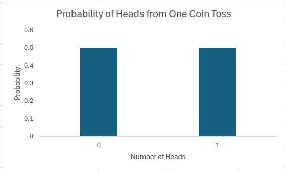
It is not the most exciting chart I have ever constructed, but it’s a start.

If I toss two coins, I get four possibilities: two Heads, a Head and a Tail, a Tail and a Head, and two Tails.

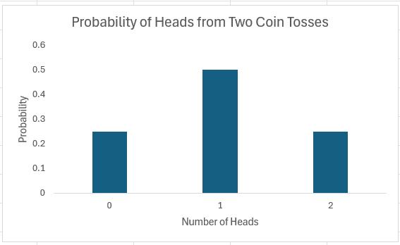
In summary, I should get two heads a quarter of the time, one head half of the time and no heads a quarter of the time. Note that (1/4) + (1/2) + (1/4) = 1. These fractions are the probabilities of the events occurring and the sum of all possible outcomes must always add up to 1.

The story is similar if we consider 16 coin tosses say:

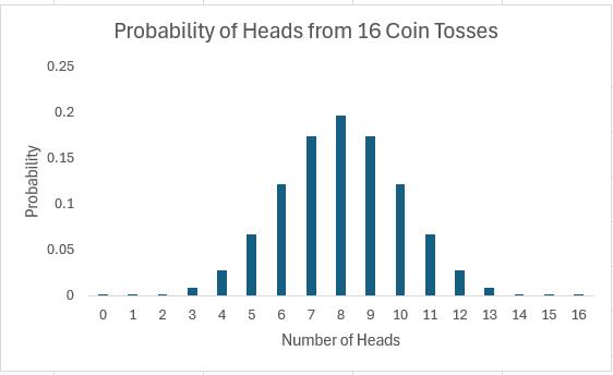
Again if you were to add up all of the individual probabilities, they would total to 1. Notice that in symmetrical distributions (such as this one) it is common for the most likely event (here, eight heads) to be the event at the midpoint.

Of course, why should we stop at 16 coin tosses?

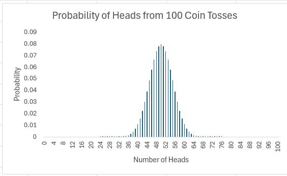
All of these charts represent probability distributions, i.e. it displays how the probabilities of certain events occurring are distributed. If we can formulate a probability distribution, we can estimate the likelihood of a particular event occurring (e.g. probability of precisely 47 heads from 100 coin tosses is 0.0666, probability of less than or equal to 25 heads occurring in 100 coin tosses is 2.82 x 10-7, etc.).

Now, I would like to ask the reader to verify this last chart. Assuming you can toss 100 coins, count the number of heads and record the outcome at one coin toss per second, it shouldn’t take you more than 4.0 X 1022 centuries to generate every permutation. Even if we were to simulate this experiment using a computer programme capable of generating many calculations a second it would not be possible. For example, in February 2012, the Japan Times announced a new computer that could compute 10,000,000,000,000,000 calculations per second. If we could use this computer, it would only take us a mere 401,969 years to perform this computation. Sorry, but I can’t afford the electricity bill.

Let’s put this all into perspective. All I am talking about here is considering 100 coin tosses. If only business were that simple. Potential outcomes for a business would be much more complex. Clearly, if we want to consider all possible outcomes, we can only do this using some sampling technique based on understanding the underlying probability distributions.

Probability Distributions

If I plotted charts for 1,000 or 10,000 coin tosses similar to the above, I would generate similarly shaped distributions. This classic distribution which only allows for two outcomes is known as the Binomial distribution and is regularly used in probabilistic analysis.

The 100 coin toss chart shows that the average (or ‘expected‘ or ‘mean‘) number of heads here is 50. This can be calculated using a weighted average in the usual way. The ‘spread’ of heads is clearly quite narrow (tapering off very sharply at less than 40 heads or greater than 60). This spread is measured by statisticians using a measure called standard deviation which is defined as the square root of the average value of the square of the difference between each possible outcome and the mean, i.e.

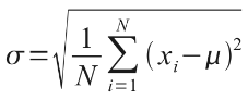
where:

? = standard deviation

N = total number of possible outcomes

? = summation

? = mean or average

xi = each outcome event (from first x₁ to last x_N)

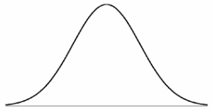
The Binomial distribution is not the most common distribution used in probability analysis: that honour belongs to the Gaussian or Normal distribution:

Generated by a complex mathematical formula, this distribution is defined by specifying the mean and standard deviation (see above). The reason it is so common is that in probability theory, the Central Limit Theorem (CLT) states that, given certain conditions, the mean of a sufficiently large number of independent random variables, each with finite mean and standard deviation, will approximate to a Normal distribution.

The Normal distribution’s population is spread as follows:

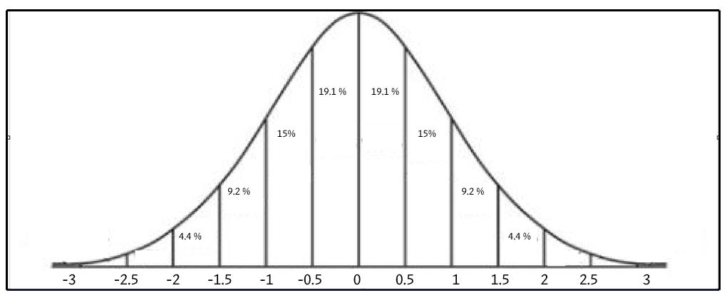
i.e. 68% of the population is within one standard deviation of the mean, 95% within two standard deviations and 99.7% within three standard deviations.

Therefore, if we know the formula to generate the probability distribution – and here I will focus on the Normal distribution – it is possible to predict the mean and range of outcomes using a sampling method.

The formula for the Normal distribution is given by

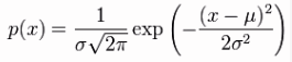
and Excel has two functions that can calculate it:

• NORMDIST(x,mean,standard_deviation,cumulative) When the last argument is set to TRUE, NORMDIST returns the cumulative probability that the observed value of a Normal random variable with specified mean and standard_deviation will be less than or equal to x. If cumulative is set to FALSE (or 0, interpreted as FALSE), NORMDIST returns the height of the bell-shaped probability density curve instead.
• NORM.DIST(x,mean,standard_deviation,cumulative) As above, but note that since Excel 2007, Microsoft has updated many of its statistical functions. To provide backward compatibility, they changed the names of their updated functions by adding periods within the name. If you are new to both of these functions, I would suggest using this variant as Microsoft has advised it may not support the former function in future versions of Excel.

The attached Excel file (or if you have problems, try this version of the Excel file for those using Excel 2007 or earlier) provides an example of how this latter Excel function can be used in practice:

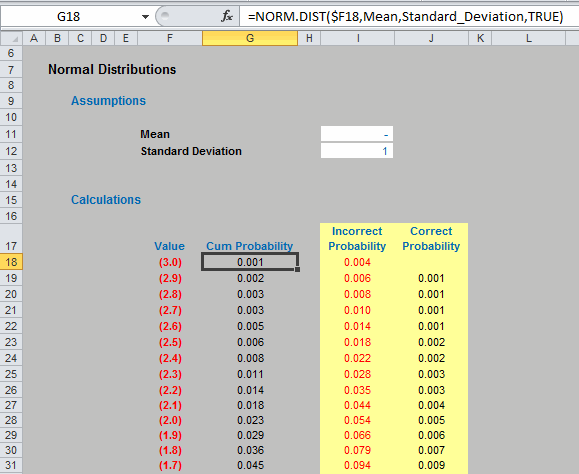
Check out the example though to see how it can catch out the inexperienced user when trying to assess just the (non-cumulative) probabilities.

Hopefully, the above has all been a useful refresher / introduction to the area, but it is now time to ask the question: how can we undertake simulations analysis in Excel..?

Simulations Analysis in Excel

Since it is clear we cannot model every possible combination / permutation of outcomes, the aim is to analyse a representative sample based on a known or assumed probability distribution.

There are various ways to sample, with the most popular approach being the “Monte Carlo” method, which involves picking data randomly (i.e. using no stratification or bias). Excel’s RAND() function picks a number between 0 and 1 randomly, which is very useful as cumulative probabilities can only range between 0 and 1.

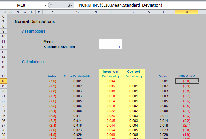
NORMINV(probability,mean,standard_deviation) and NORM.INV(probability,mean,standard_deviation) return the value x such that the cumulative probability specified (probability) represents the observed value of a Normal random variable with specified mean and standard_deviation is less than or equal to x. In essence this is the inverse function of NORM.DIST(x,mean,standard_deviation,TRUE):

Now, we are in business if we assume our variable is Normally distributed. We can get Excel to pick a random number between 0 and 1, and for a given mean and standard deviation, generate a particular outcome appropriate to the probability distribution specified, which can then be used in the model as in the following illustration:

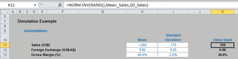
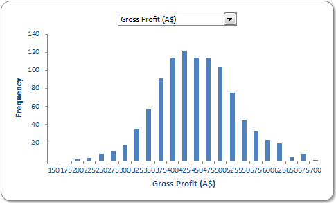
Here, three variables, Sales, Foreign Exchange and Gross Margin all employ the NORM.INV function to generate the assumptions needed to calculate the Gross Profit. We can run the simulation a given number of times by running a simple one-dimensional Data Table (for more information on Data Tables, please see Being Sensitive With Data Tables).

The actual approach is a little crafty though:

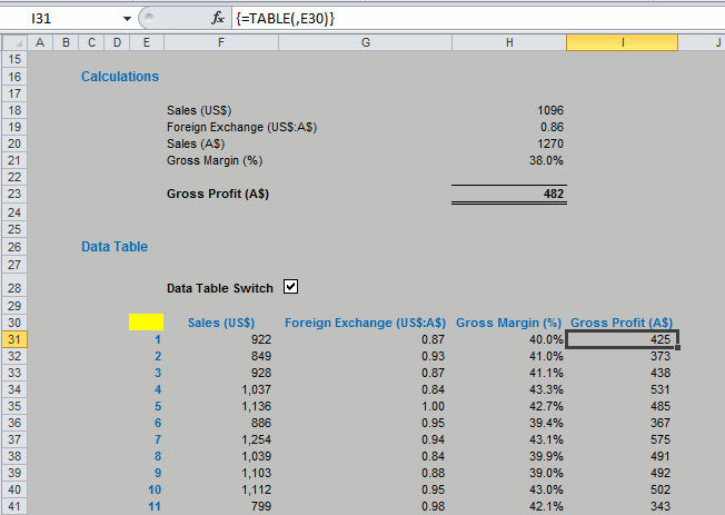
Since the variables use the RAND function to generate random numbers, each time the end user presses ‘ENTER’ or hits ‘F9?, the variables will recalculate (this quality is known as volatility). Therefore, since each Data Table entry causes the model to recalculate for each column input, the values will change automatically. On this basis, note that the column input cell in the example above refers to E30 (the cell highlighted in yellow) which is unused by any formula on the spreadsheet.

The example in the attached Excel file (or again, this modified Excel file for Excel 2007 and earlier users) has 1,000 rows (i.e. 1,000 simulations). Since the variables have been generated randomly, this is a simple Monte Carlo simulation – no fancy software or macros required!

It only requires a quick collation step to summarise the outputs graphically:

Please see the file for more details.

Word to the Wise

There are three key issues surrounding this article:

1. Not all variables are Normally distributed. Consequently, using the NORM.INV function may be inappropriate for other probability distributions;
2. The above example has assumed all variables are independent. If there are interrelationships or correlations between inputs, this simple approach would need to be revised accordingly; and
3. Working with probabilities is notoriously counter-intuitive. Take care with interpreting results and always remember that the results only represent a sample of possible outcomes (the sample size may be too small for extrapolation to the entire population). If in doubt, consult an expert!