
Credit where credit’s due…
Never has it been clearer than in the current global economy that cash is king. This article considers the practical issues surrounding modelling working capital adjustments. By Liam Bastick, director with SumProduct Pty Ltd.
Query
I have forecast income and expenditure items for the company’s Income Statement. What tips can you provide for deriving cash flow figures from these projections?
Advice
Let’s start at the beginning: please feel free to use the attached Excel file to help clarify the ideas discussed below.
Consider the following example:
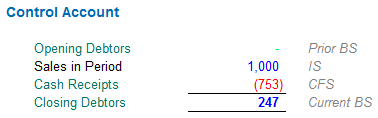
Imagine a company just starts off in business (i.e. has no amounts due) and generates sales of $1,000 in the period. At the end of the period, assuming no bad debts, $753 has been paid, leaving a closing debtor balance of $247. This difference is what I refer to as the working capital adjustment.
If we had modelled the sales of $1,000 in the period, how might we generate the cash receipts forecast such that is assumptions changed, the receipts would calculate appropriately?
Clearly, if we are given the closing debtor balances, the problem becomes trivial, so I will assume that this is not so. Therefore, I am going to consider an alternative approach and some of the associated underlying issues that need to be considered when modelling.
At the risk of teaching the accountants in the audience to suck eggs, let me first derive an alternative method.
Let’s assume that the sales accrue evenly over the period of time and for the sake of this example, that period is one year (365 days). Presuming (i) all sales are made on credit terms, (ii) all customers pay their invoices on the day the amounts fall due and (iii) no bad debts are incurred, this can be reflected graphically as follows:
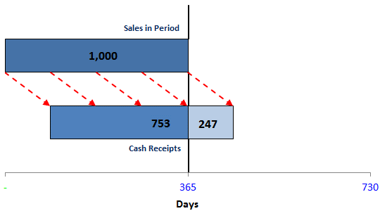
Clearly, the credit period is the “gap” at the beginning of the time period, i.e. 247/1000 x 365 days = 90 days. This can be represented formulaically as:
Days Receivable = (Closing Debtors x Days in Period) / Sales in Period
Rearranging, this becomes:
Closing Debtors = (Sales in Period x Days Receivable) / Days in Period,
e.g. in our example: 247 = (1000 x 90) / 365.
Therefore, in modelling, we often set the number of days receivable (and days payable) as key assumptions for cash flow forecasting.
However, it’s not always as simple as that. Let me explain. Consider we are planning to build a monthly model (assuming 30 days in a month) and sales for the month are again $1,000. Debtor days remain at 90 days.
Based on these calculations, we would generate the following control account:
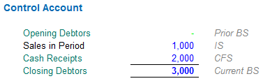
Erm, that’s right: make sales of $1,000 and have $3,000 (= 90/30 x 365) owing to you by the end of the month. Also, the company pays $2,000 to customers a reclaimable $2 for each $1 spent. That’s nonsense – and yet, as an experienced model auditor I have seen this erroneous calculation crop up on a regular basis…
Monthly Forecasting
The problem is, in this current economic climate most businesses want to prepare monthly – sometimes weekly and even daily – cash flow projections. Clearly, if the days receivable or days payable assumption exceeds the number of days in each forecast period this approach is inappropriate and will lead to calculation errors.
So what do we do in this situation..?
For example, in a monthly model, if payments are made exactly one month or two months or three months later (and so on), the resolution is simple: the receipts can be calculated using a simple OFFSET (displacement) formula.
Therefore, let’s complicate the scenario slightly. Imagine we are building a monthly forecast model, but that the days receivable are 75. For the purposes of keeping this article reasonably brief, I will simplify the problem by assuming an average number of days in a month (say, 30). Using this simplifying assumption, this will mean that payments are made on average 2.5 (2.5 = 75 / 30) months after the sale has been made.
That 2.5 months figure is important. The integer part (2) denotes how many complete months (including the current month) have sales payments outstanding. The residual (0.5) shows the proportion of the month preceding these complete months that is also outstanding. With this borne in mind, the OFFSET function can now come to the rescue, viz.
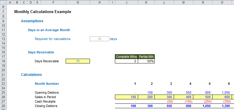
In this illustration (above), cells J18 and K18 break the number of days receivable (cell G18) into the number of whole months and residual proportion respectively, assuming that each month has 30 days (cell H13).
The key formula here is the calculation for Closing Debtors (Cash Receipts is simply the balancing figure). For example, the formula in cell J28 (above) is:
=IF($J$18,SUM(OFFSET(J26,,,1,-MIN($J$18,J$23))),)
+IF(J$23-$J$18<=0,,OFFSET(J26,,-$J$18)*$K$18)
It may seem a little complex upon first inspection, but it’s not as bad as it seems. Essentially, there are two parts to this formula identified by the two added IF statements:
1. IF($J$18,SUM(OFFSET(J26,,,1,-MIN($J$18,J$23))),) considers the completed number of months where sales remain outstanding and adds up the sales for these periods. This approach has been discussed previously in detail in the Simple Depreciation Example detailed in my OFFSET article.
In essence, this part of the formula checks that the number of completed months is not zero (in this case the amount is just zero), and assuming this is not the case, it sums the sales for the relevant number of completed months (i.e. starts with the current month and then considers the sales in previous months, working from right to left in the spreadsheet). The MIN formula is required to ensure that the model does not try to include periods prior to the beginning of the forecast period).
2. IF(J$23-$J$18<=0,,OFFSET(J26,,-$J$18)*$K$18) considers the residual (remaining) amount for the month before the earliest completed month. For example, if the credit period is 2.5 months and the current month is April, then March and April will be “whole months” where no payment has been received, with half of February’s monies still outstanding too.
The reason for the IF statement here is to prevent calculations considering periods before the beginning of the forecast period.
To clarify, consider the Closing Debtor figure of $1,050 in Period 5 (above, cell N28 in the illustration). This is calculated as the sales for Periods 4 and 5 (400 + 500 respectively), plus half of the Period 3 sales (300 x 0.5 = 150), i.e. 400 + 500 + 150 = 1,050.
More Complex Scenarios
It only gets more complicated. What if payments are not made evenly? Or that some sales are written off as payments are never made (i.e. bad debts)? Actually, we have covered this scenario in a previous article.
Depreciation..?
Think about it: depreciation arises when cash is laid out in one period, but the costs are allocated over multiple periods. Debtors arise when sales are made in one period, but the cash receipts are allocated over multiple periods. It’s the same logic, just different labelling!
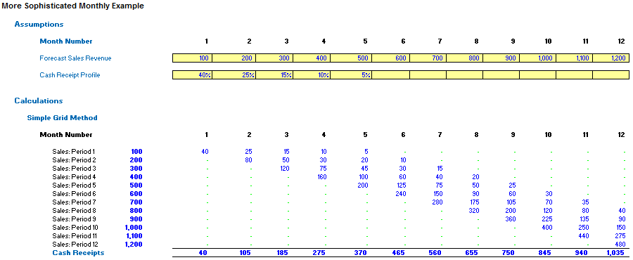
The calculations can be reviewed in depth in the attached Excel file, but what can be clearly seen is the similarity to a depreciation calculation. In this illustration, the Cash Receipt Profile percentages do not add up to 100%. This is deliberate – the missing 5% is the assumed bad debt here.
Word to the Wise
This article is intended to be a starting point for considering the modelling issues surrounding working capital adjustments. You can complicate matters further by considering any or all of the following:
- What proportion of sales / costs is made on credit terms?
- Calculate extended credit periods using the actual number of days in each month rather than using an average number
- Calculations using average days receivable (payable) based on both the opening and closing debtor (creditor) balances
- How adjustments differ by considering public holidays, the number of working days, seasonality and cyclicality etc.
- Sales / costs are invoiced in a foreign currency and the exchange rate differs over time
- Factoring in segmental reporting, e.g. based on customer profitability / size / geography etc.
- Infrastructure projects often have large one-off payments that will occur on specific dates (here you just need to calculate which month the payment will occur in).
Happy modelling!