Appreciation of Depreciation
This article considers an issue most modellers have to resolve on a regular basis. By Liam Bastick, director with SumProduct Pty Ltd.
Query
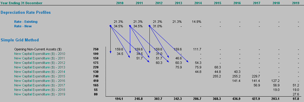
How do you model the total depreciation charge for a given period (yellow cells in illustration, below)?
Advice
Having reviewed models for many years, I’ve seen that most modellers can build this as long as the economic life is a whole number.

However, I am going to offer a solution that allows for non-integer economic lives whilst making the following simplifying assumptions:
- No residual values (i.e. the depreciable amount is the purchase price);
- No change of economic life;
- No change of depreciation method; and
- A full period’s depreciation is charged in the period of acquisition.
The key thing is to identify the depreciation rate profile (i.e. the percentage of the purchase price depreciated each period). This is true whatever the depreciation method, and can either be calculated or typed in. For straight line depreciation, this is not as simple as taking the reciprocal of economic life (i.e. 1 / economic life), since we need to ensure that:
- We do not over-depreciate (i.e. the aggregation of the percentages does not exceed 100%);
- We ensure that if the economic life is not a positive number we do not calculate nonsensical percentages (e.g. -5%) or calculate #DIV/0! errors.
Hence, the formula in principle to use for straight-line depreciation would be:
=IF(Economic_Life<=0,0,MIN(1/Economic_Life,100%-SUM(Percentages_So_Far)))
The attached Excel file demonstrates how to construct this in practice.

So, in the attached illustration, the economic life for new capital expenditure was assumed to be 2.9 years. 1/2.9 = 34.5% (approx.), and this is the rate used for the first two years. However, in the third year (2012), only 31.0% remains (since 100.0% – (2 x 34.5%) = 31.0%), and this is the amount used. Thereafter, all amounts are zero. From here, it is relatively straightforward to create a simple grid that calculates how capital expenditure is depreciated each period using these percentages:

I have included in the Excel file a simple way (which is highly transparent) and a more sophisticated way (which allows the formula in the top left cell of the grid to be copied across and down). The problem with this approach is depending on the number of asset classes, number of periods, whether you are calculating depreciation for tangibles and intangibles and / or accounting and tax. Clearly, this can increase the size of the Excel file almost exponentially.
This is where the challenge comes in: is there a way of avoiding the grid? There are straightforward ways of shortcutting the above when the percentage is the same amount in each period. Most of these methods fall over, however, when the percentage changes.
Reverse Ticker Method
The objective is to calculate the depreciation for each period knowing the depreciation rate profile and the capital expenditure, viz.

In the above example, the 2010 depreciation charge is simple: =J30*J45. The 2011 charge has four precedents:

Here, the calculation is =(J30*K45)+(K30*J45). It gets slightly more sophisticated for 2012:

In this example, the formula is =(J30*L45)+(K30*K45)+(L30*J45).
Clearly, these formulae will become more and more awkward to construct. Further, the formulae are not consistent across a row, which makes the model more difficult to understand for developer and user alike. But there’s a trick: what if we reversed the percentage profile?

Row 83 has been displayed reversing the order of the depreciation rate profile, using the OFFSET function (see April 2009 Insight article for a full discussion on this very useful Excel function) and a counter (row 18 in this example):
=OFFSET($T45,0,-J$18)
(This simple formula merely references the cell x columns to the left of cell T45, where x is the value in cell J18.)
A consistent formula can then be constructed in row 86, using OFFSET again and the SUMPRODUCT function (see July 2009’s Insight article on Multiple Criteria):
=SUMPRODUCT(OFFSET($J30,0,0,1,J$18),OFFSET($S83,0,0,1,-J$18))
This formula might look horrible to start off with, but it’s not that bad when considered systematically.
OFFSET($J30,0,0,1,J$18) means “select x cells in a row starting at J30, where x is the number in J18”.
OFFSET($S83,0,0,1,-J$18) means “select x cells in a row ending at S83, where x is the number in J18”.
Hence the equation in J86 becomes (J$18=1):
=SUMPRODUCT(OFFSET($J30,0,0,1,J$18),OFFSET($S83,0,0,1,-J$18))
=SUMPRODUCT($J30,$S83)
=$J30*$S83
Whereas the equation in M86 becomes (M$18=4):
=SUMPRODUCT(OFFSET($J30,0,0,1,M$18),OFFSET($S83,0,0,1,-M$18))
=SUMPRODUCT($J30:M30,P83:$S83)
=($J30*P83)+(K30*Q83)+(L30*R83)+(M30*$S83)
which is in essence the calculation explained above. Once you master this technique I assure you that you will never look back!
If you have a query for this section, please feel free to drop Liam a line at liam.bastick@sumproduct.com or visit the website www.sumproduct.com

