
Power Pivot Principles: Slicers for Columns – Part 2
19 January 2021
Welcome back to the Power Pivot Principles blog. This week, we will continue to talk about slicers for columns.
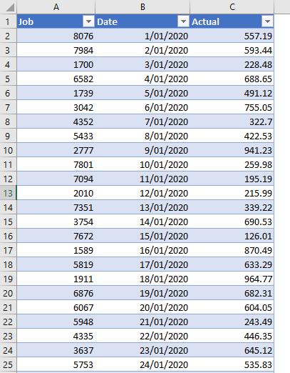
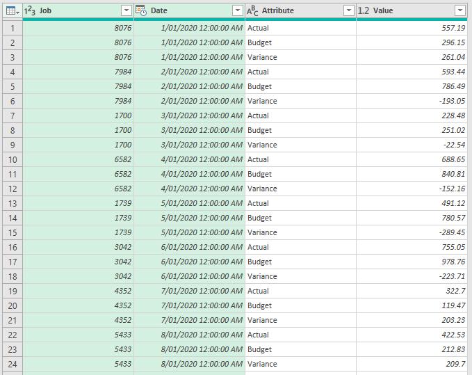
Last week, using Power Query, we combined and transformed the Actual revenue table
and the Budget revenue table
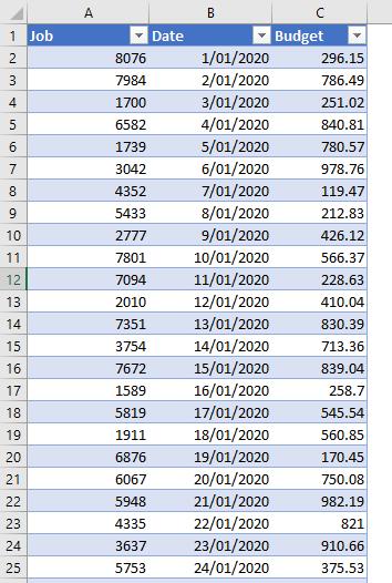
to one Data table like the one below:
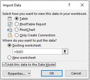
We load this table to Excel, from the ‘Queries & Connections’ panel, right-click on the Data table and select ‘Load To…’. An ‘Import Data’ dialog will appear. In here, we will tick the box ‘Add this data to the Data Model’.
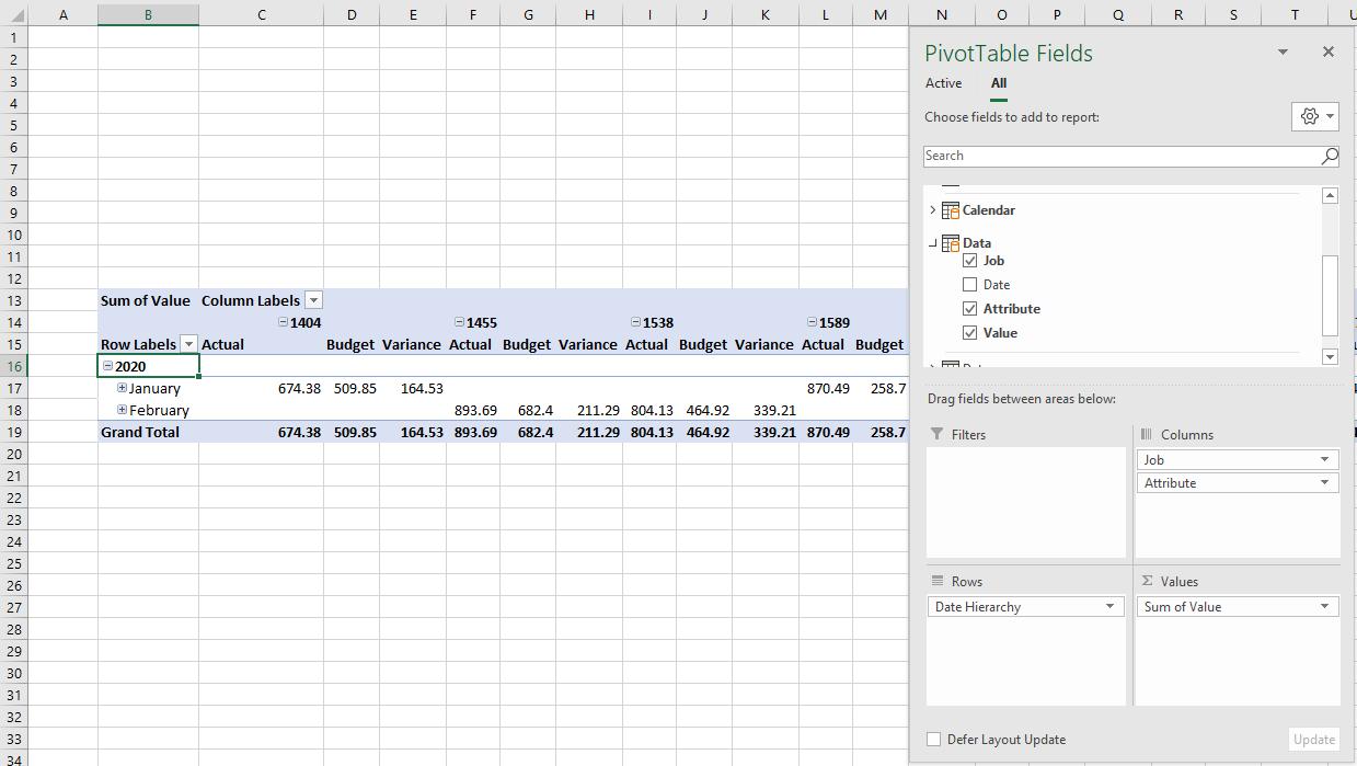
In the Power Pivot Data Model, we will create a Calendar table and link the Date columns of the tables to form a relationship between them. Then, we will create a PivotTable and load this to a new worksheet in Excel and drag the fields to the appropriate areas as illustrated below:
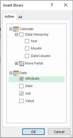
Next, we will create slicers. Navigate to the ‘PivotTable Analyze’ contextual tab on the Ribbon and select ‘Insert Slicers’. In the ‘Insert Slicers’ dialog, tick the Job and Attribute boxes.
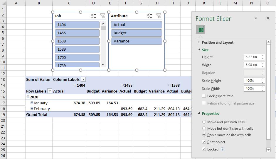
We will have the slicers displayed on top of the PivotTable. Select both slicers, right-click and choose ‘Size and Properties’ then check ‘Don’t move or size with cells’ to fix the slicers in their places. You can read more about working with slicers here.
Now, we’re good to go…
Stay tuned for our next post on Power Pivot in the Blog section. In the meantime, please remember we have training in Power Pivot which you can find out more about here. If you wish to catch up on past articles in the meantime, you can find all of our Past Power Pivot blogs here.