Slicer of Good Fortune

This month, in our series of articles providing solutions to common issues encountered by finance professionals, Liam Bastick, director (and Excel MVP) with SumProduct Pty Ltd, takes a look at how slicers can make your outputs look more professional.

Query

Should I use slicers for my output sheet(s)?  Are there any potential issues to watch out for?

Advice

I am going to assume you are happy how PivotTables work.  If not, please feel refer back to Pivotal PivotTable, May 2009’s Insight article >here. 

In earlier versions of Microsoft Excel, you can use report filters to filter data in a PivotTable report, but it is not easy to see the current filtering state when you filter on multiple items.  In Microsoft Excel 2010 and later versions (i.e. from when slicers were introduced), you have the option to use slicers to filter the data.  Slicers provide buttons that you can click to filter PivotTable data.  In addition to quick filtering, slicers also indicate the current filtering state, which makes it easy to understand what exactly is shown in a filtered PivotTable report.  You can even filter on data that isn’t explicitly on of the dimensions on a PivotTable.

You can actually use slicers with Tables, PivotTables, PivotCharts and Power Pivot’s PivotTables.  Here, I am just going to focus on PivotTables, but the idea remains similar for all similar circumstances.

To illustrate how they work, I am using the attached Excel file as my muse.  In it, I have some data:

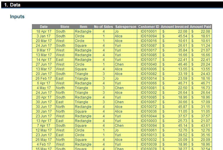
I have created a PivotTable by selecting any cell in this contiguous range and then from the ‘Insert’ tab on the Ribbon clicking on ‘PivotTable’ (the rather intuitive keyboard shortcut ALT + N + V):

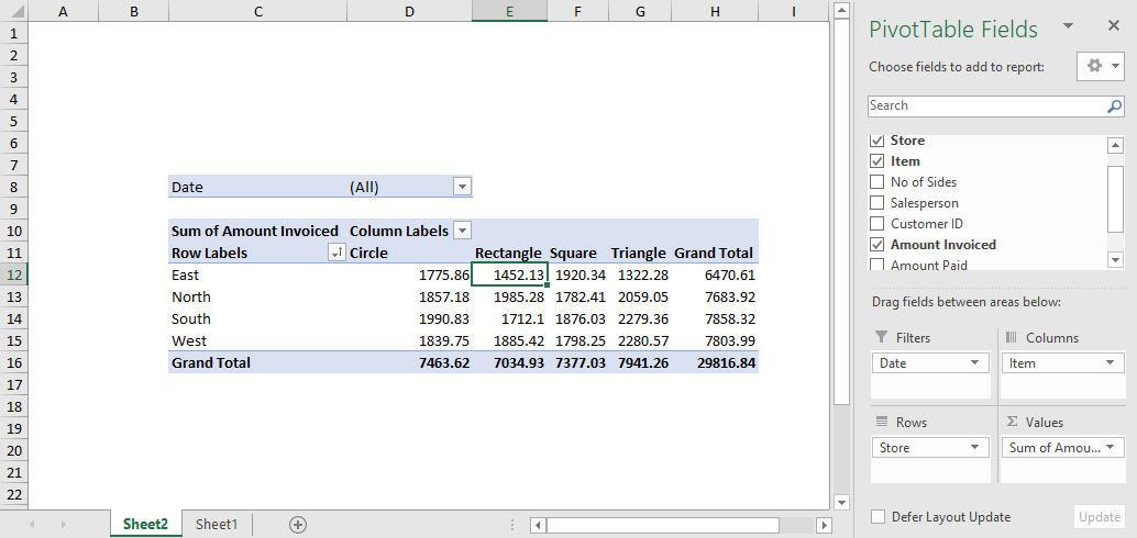
You can clearly see the filters (drop down arrows) alongside Date, Store and Item.  The filters can replace these.  However, before I do that, let’s do some housekeeping.  I can make the row and column headers much more informative by doing very little.  All I have to do is select a cell inside the PivotTable and then from the context Ribbon (i.e. with PivotTable Tools tabs visible), select ‘Show in Tabular Form’ from the dropdown menu in ‘Report Layout’ in the ‘Layout’ group of the ‘Design’ tab (ALT + JY + P + T):  

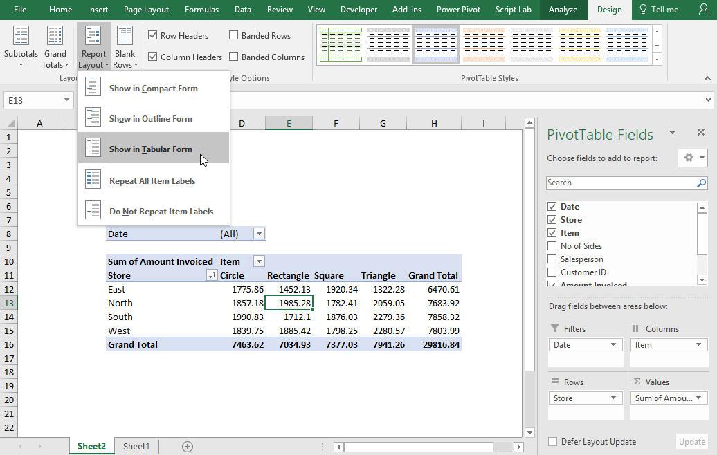
See how Item and Store are now displayed? It’s a good start, but we can go further.

Formatting in PivotTables has always been a pain in the proverbials.  Microsoft has claimed since March 2016 that they have finally fixed this though – and since they made this claim I have failed to generate a counterexample.  The trick is you must have an unfiltered table with row and column totals visible and format everything the same:

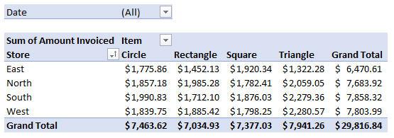
Easy!  One other thing though.  It has been stipulated that I should report my stores in a particular order, namely, “North”, “South”, “East” and “West”.  This is neither alphabetical order nor reverse alphabetical order.  How can I do this?

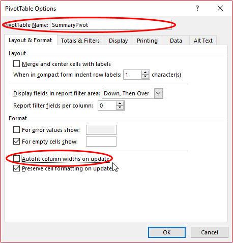
You can drag and drop the labels but this is not an ideal solution.  There is a better way.  First, right-click inside the PivotTable and select ‘PivotTable Options…’ from the context shortcut menu.  This reveals the ‘PivotTable Options’ dialog box.  On the first tab, ‘Layout & Format’, we may as well rename the PivotTable and uncheck ‘Autofit column widths on update’ (which prevents columns from continually resizing automatically) viz.

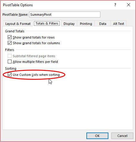
Now, let’s go to the ‘Totals & Filters’ tab and ensure that the ‘Use Custom Lists when sorting’ checkbox is enabled:

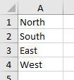
After we have clicked ‘OK’, I will now create a Custom List as follows.  It’s very easy.  Simply type your list in Excel and then highlight it:

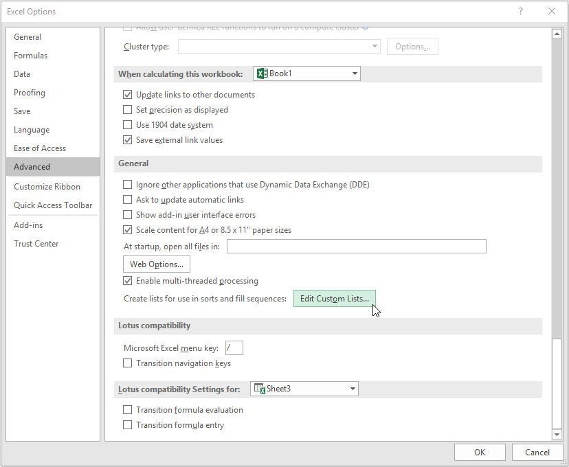
Then, go to File -> Options and then select ‘Advanced’ from the left-hand column.  Scroll down the right-hand window pane until you locate the ‘Edit Custom Lists…’ button in the ‘General’ section:

Click on this button and then

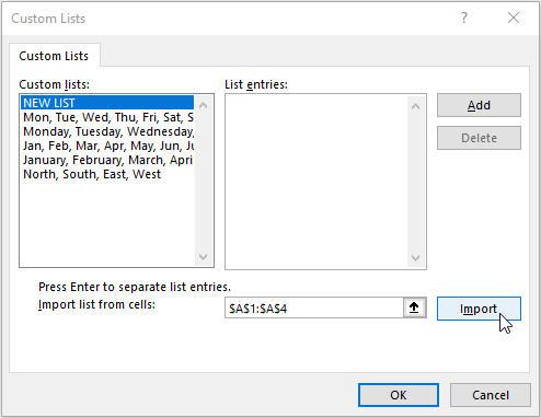
See how the cells populate the range box?  Simply click the ‘Import’ button and “North”, “South”, “East” and “West” is now a custom list with this order duly noted.  After we have clicked ‘OK’ (and you may need to refresh the PivotTable), you should now get:

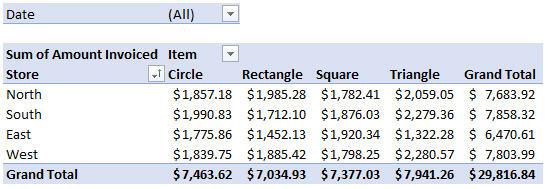
This order will also dictate the order in slicers – so I suppose it’s time I finally get around to introducing them!

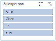
They’re very easy – simply click inside the PivotTable once more and then from the context Ribbon (i.e. with PivotTable Tools tabs visible), select ‘Insert Slicer’ in the ‘Filter’ group of the ‘Analyze’ tab (ALT + JT + SF):  

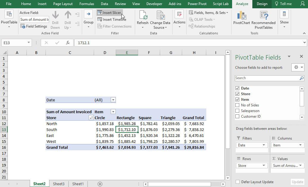
Depending upon your screen resolution, ‘Insert Slicer’ may appear differently to how it is illustrated (above).  Select several slicers and try to drag them to approximately where you want to have them positioned.  Holding the ALT button down as you drag the slicer with the mouse makes the slicer ‘snap’ to the Excel grid if that helps. 

I recommend putting slicers either to the left or above a PivotTable.  This is because a PivotTable’s dimensions will change as you filter for different criteria.  A PivotTable will never encroach to the left or above.  It is for this reason why you should also take care if you place more than one PivotTable on the same worksheet.

When positioning more than one slicer, concentrate on getting the first slicer positioned correctly and then ensure second and subsequent slicers are ‘touching’ the slicer immediately to its left.  Don’t worry about any other alignment:

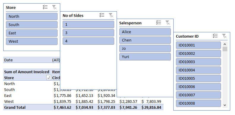
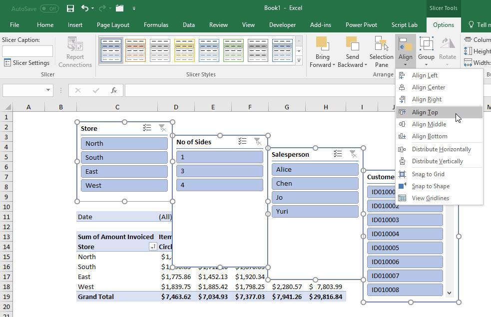
The Store slicer has been resized and positioned where I want it, but the other are just placed so that they are ‘side by side’.  Next, I select all four by clicking on the first slicer, then hold the SHIFT button down and clicking on the remainder.  With these slicers all selected, I now go to the context Ribbon (i.e. with the ‘Slicer Tools’ tab visible) and select ‘Align Top’ from the ‘Align’ dropdown menu in the ‘Arrange’ group of the ‘Options’ tab (ALT + JO + AA + T):  

Next, I click on my first slicer and note its dimensions as follows:

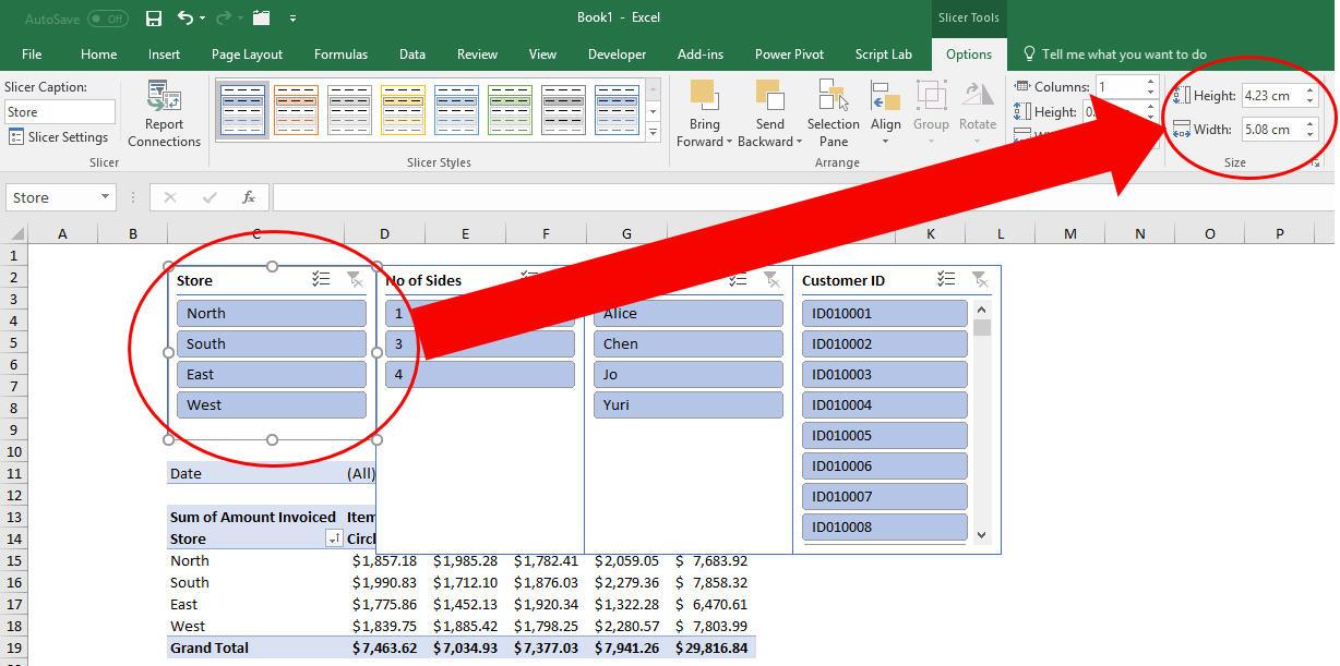
Then, select each slicer in turn and modify the height and width accordingly (I decided to make the last slicer twice the width):

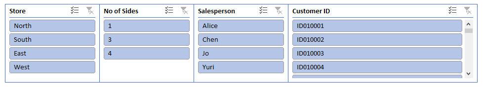
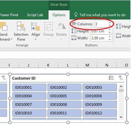
See how they line up?  My last slicer has many possible selections, so I click on the Customer ID slicer and then change the number of columns in the ‘Buttons’ group: 

There’s more.  We have spent all of this time lining up the slicers.  We had better make sure they don’t move!  To ensure they do not move, select all of the slicers and then right-click and select ‘Size and Properties…’ from the context shortcut menu.  In the ‘Format Slicer’ pane, select the ‘Don’t move or size with cells’ option button in the ‘Properties’ section as pictured:

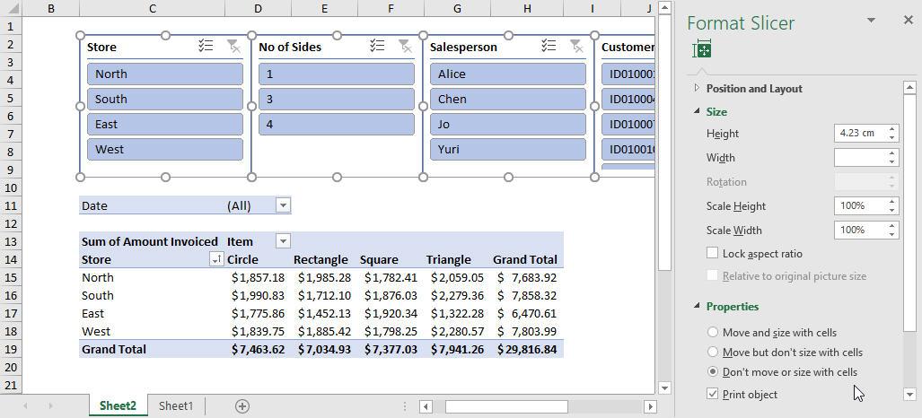
Even if the columns or rows are modified in some fashion, the relative positioning of our slicers will be retained. 

There’s one other thing to do with the slicers: we want to ensure we cannot select impossible combinations, e.g. four-sided triangles.  This may be prevented by again selecting all of the slicers, right-click and then select ‘Slicer Settings…’ from the context shortcut menu.  Then, uncheck ‘Show items deleted from the data source’, ‘Show items with no data last’ and ‘Visually indicate items with no data’ (in that order, otherwise this will not be possible).  Then, check ‘Hide items with no data’:

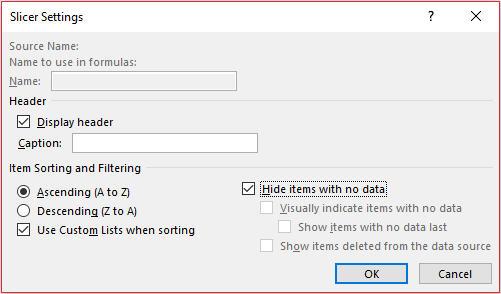
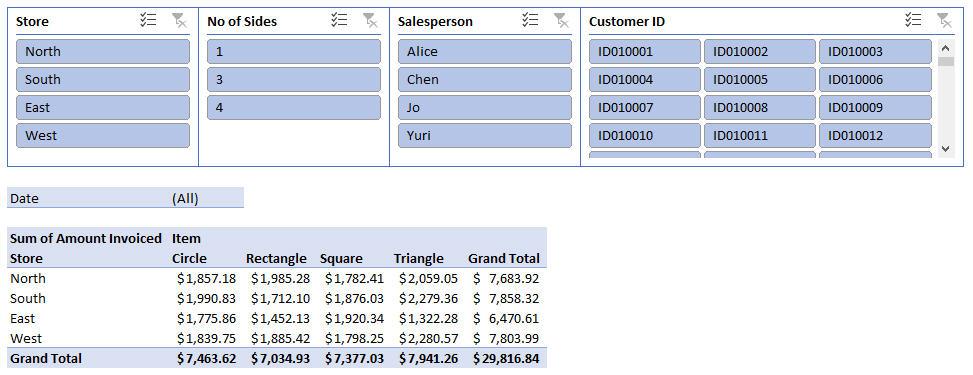
Now, the slicers will behave themselves.

At this stage, the filter dropdown arrows are still visible on the PivotTable.  There is no Excel option to hide these.  Running the following macro will remove them:

This macro will remove the filters from all PivotTables on a particular worksheet (the ‘100’ is arbitrary – it assumes there’s no more than 100 PivotTables on the sheet!).

Voila!  No filter arrows.  This forces end users to use the slicers to make their selections.

Now my macro works for multiple PivotTables.  However, if I add in more PivotTables, you will notice that initially, the slicers only work for the PivotTable that was selected when the slicer was inserted.  This problem is not insurmountable, but it can be cumbersome if you have multiple slicers as you have to modify each slicer individually. 

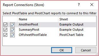
To do this right click on a slicer and select ‘Report Connections…’ from the context shortcut menu and select the Pivot Tables you wish to affect:

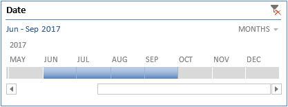
There is another type of slicer you may add too.  First appearing in Excel 2013, the Timeline feature allows you to select a date range (which must be contiguous).  It isn’t compatible with earlier versions of Excel, but it does look good in a dashboard when available:

To insert a timeline, simply click inside the PivotTable once more and then from the context Ribbon (i.e. with PivotTable Tools tabs visible), select ‘Insert Timeline’ in the ‘Filter’ group of the ‘Analyze’ tab (ALT + JT + ST):  

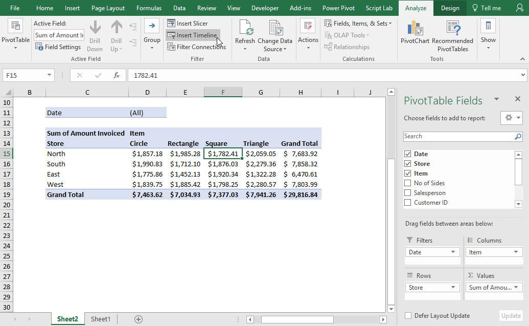
Depending upon your screen resolution, ‘Insert Timeline’ may appear differently to how it is illustrated (above).  There is a problem inherent with timelines though.

When you try to align slicers and timelines using ‘Align’ they often don’t appear to be quite right:

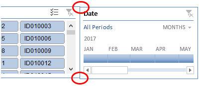
If the screenshot were to be printed, you would see that they do align.  The problem is, they don’t appear to align on screen.  If you do line it up by eye on screen instead, they will not align if printed.  It appears to be a bug, but I wouldn’t hold your breath awaiting a fix any time soon.

Nonetheless, with multiple PivotTable, PivotCharts, Tables, slicers and timelines, you can make great interactive dashboards in your Excel workbooks:

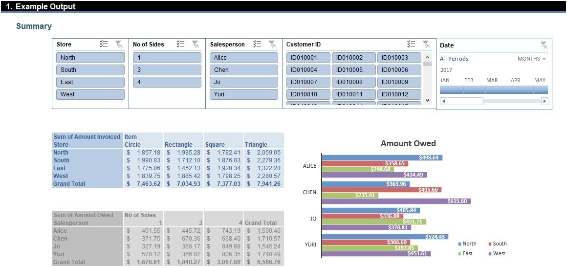
You can check out this dashboard example in the attached Excel workbook.

Word to the Wise

Sometimes, you cannot seem to add a slicer or timeline.  This can be because you are working in the wrong file format (.xls will not support these features) or because a Table or PivotTable has corrupted.

In this case, you can either rebuild the PivotTable (i.e. create a new one) or else you can try to repair the old one.  To repair, save the file as an .xls file (noting any compatibility issues) and then re-saving it back as an .xlsx or .xlsm file.  This may “kick start” the PivotTable, but I offer no guarantees!

If you have a query for the Spreadsheet Skills section, please feel free to drop Liam a line at liam.bastick@sumproduct.com or visit the SumProduct website.