
Power Pivot Principles: RELATED vs LOOKUPVALUE
26 May 2020
Welcome back to the Power Pivot Principles blog. This week, let’s discuss the difference between the RELATED and LOOKUPVALUE functions.
Both the RELATED and LOOKUPVALUE functions in DAX work similarly to a LOOKUP function in Excel. We talked about LOOKUPVALUE a while ago; this is a simple function which returns the value in a given result column for the row that meets all the criteria specified by search column and search value:
LOOKUPVALUE(result_columnName,search_columnName,search_value[, search_columnName, search_value]…[,alternateResult])
Similarly, the RELATED function in DAX returns a single value that is related to the current row:
RELATED(column)
The RELATED function’s syntax looks simple, while LOOKUPVALUE’s seems complicated. This is because when the RELATED function performs a lookup, it examines all values in the specific table regardless of any filters that may have been applied; therefore, a relationship between data table is a prerequisite. Meanwhile, LOOKUPVALUE does not depend upon a relationship to work, as search and result column names are defined in the formula.
Let’s make this clear by continuing the example we have used in the RELATED function article here.
To recap, we have a data about daily quantity sales of several products in a supermarket over three years as shown below:

In another worksheet, we have the data for the price per unit of those products:
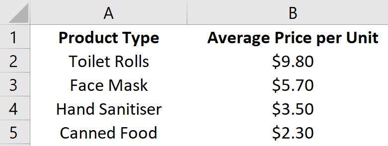
To facilitate analysis, we need to figure out the revenue, which equals
Quantity Sold x Average Price per Unit.
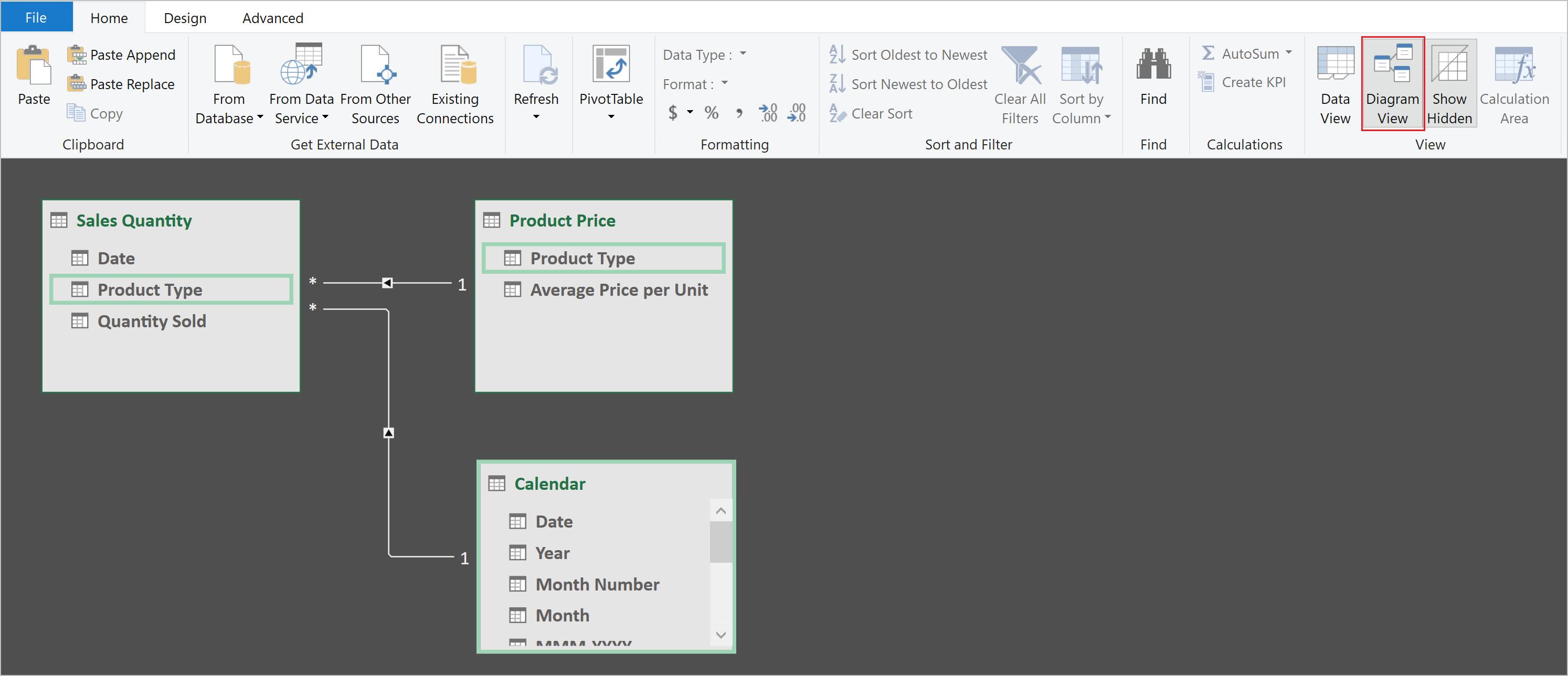
These two fields, unfortunately, lie in two different places, and we need to bring them into one table. We load the data to Power Pivot Data Model, rename the two tables as ‘Sales Quantity’ and ‘Product Price’ respectively. We can also add a Calendar Table, which will later be used in PivotTable.
For the RELATED function to work, we need to define the relationships amongst our data tables. By switching to ‘Diagram View’ in the Home tab, we drag the ‘Product Type’ field to connect two tables, ‘Sales Quantity’ and ‘Product Price’, simultaneously, as well as the ‘Date’ field of ‘Sales Quantity’ and ‘Calendar’:
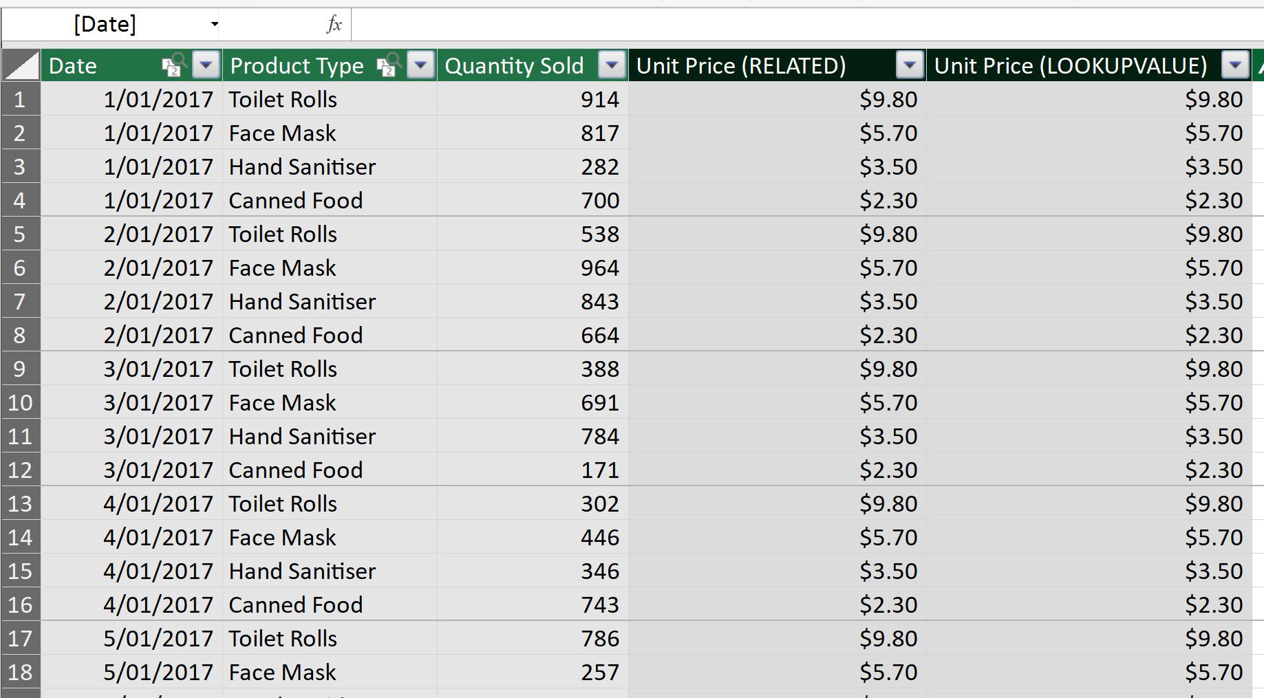
Switching back to ‘Data View’, we add new calculated columns to find ‘Average Price Per Unit’, by looking up the ‘Average Price per Unit’ in the ‘Product Price’ table to match the ‘Product Type’, to compare the two functions:
- ‘Unit Price (RELATED)’:
=RELATED(‘Product Price’[Average Price per Unit])

- ‘Unit Price (LOOKUPVALUE)’:
=LOOKUPVALUE('Product Price'[Average Price per Unit],'Product Price'[Product Type],'Sales Quantity'[Product Type])
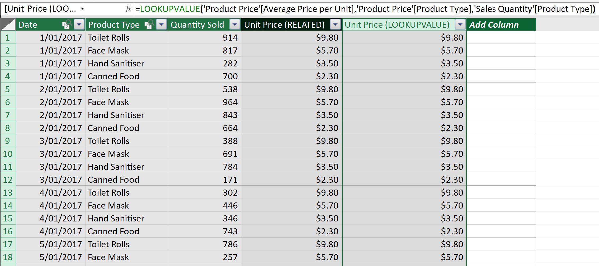
Both functions work fine. Now, if we switch to ‘Diagram view’ and remove the relationships between the data tables:
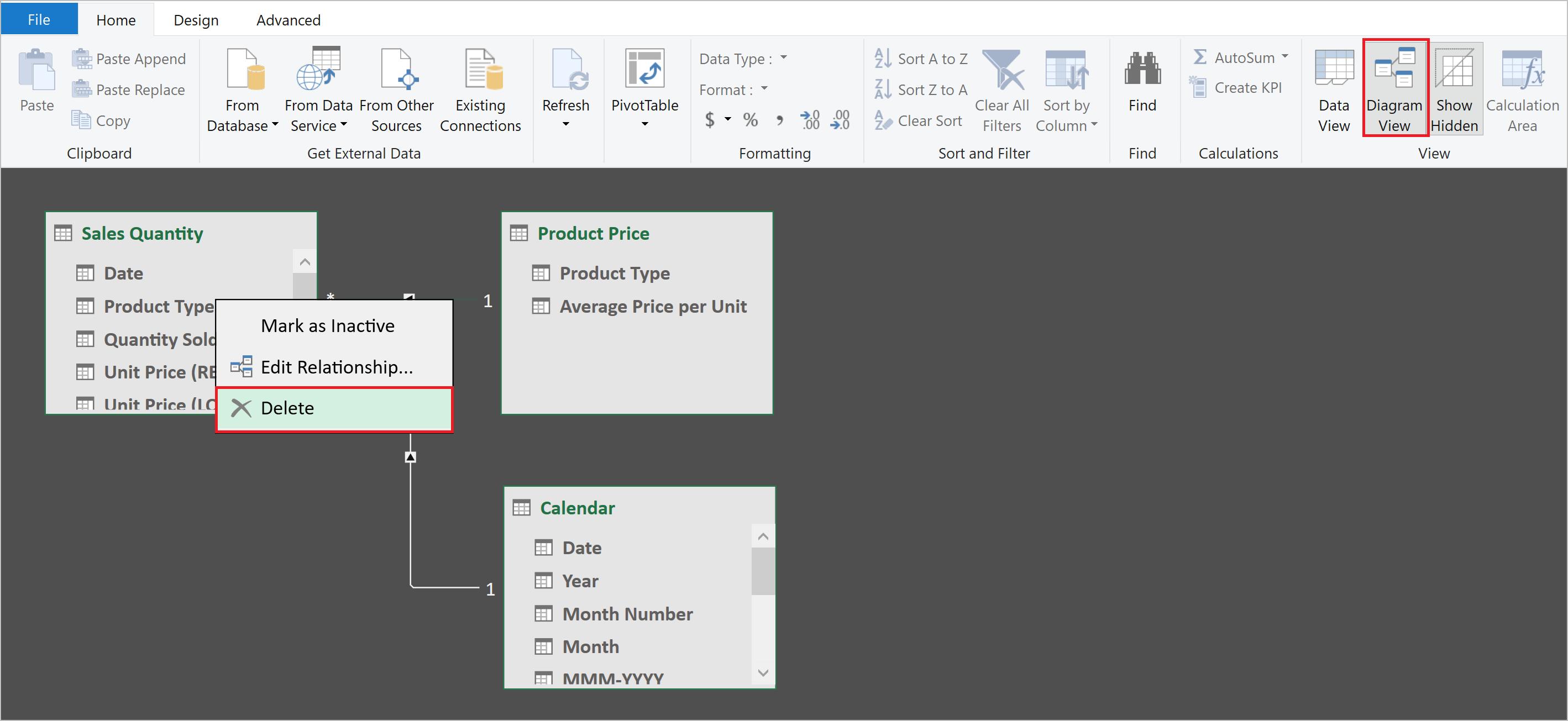
Going back to ‘Data view’, we see that the ‘Unit Price (RELATED)’ column shows all #ERROR! This is because there is nothing related between the tables, so RELATED function cannot perform the lookup. Meanwhile, the no-relationship data model has no impact upon the ‘Unit Price (LOOKUPVALUE)’ column:

If we reconnect the relationships between those tables, the #ERROR will disappear!
That’s it for this week!
Stay tuned for our next post on Power Pivot in the Blog section. In the meantime, please remember we have training in Power Pivot which you can find out more about here. If you wish to catch up on past articles in the meantime, you can find all of our Past Power Pivot blogs here.