Power Pivot Principles: Introducing the Function LOOKUPVALUE

Welcome back to the Power Pivot Principles blog.  Before we learn more functions for parent-child hierarchies in DAX, this week, we are going to look aside at one function of looking up values in DAX.

This week, we are going to look at the function: LOOKUPVALUE.  This is a simple function which returns the value in a given result column for the row that meets all the criteria specified by search column and search value.

The LOOKUPVALUE function uses the following syntax to operate:

where:

• <result_columnName> is the name of an existing column that contains the value you want to return.  The column must be named using standard DAX syntax, usually, fully qualified.  It cannot be an expression
• <search_columnName> is the name of an existing column, in the same table as result_columnName or in a related table, over which the look-up is performed.  The column must be named using standard DAX syntax, usually, fully qualified.  It cannot be an expression
• <search_value> is a scalar expression that does not refer to any column in the same table being searched
• <alternateResult> (optional) is the value returned when the context for result_columnName has been filtered down to zero or more than one distinct value.  When not provided, the function wouldreturn BLANK() in such instances.

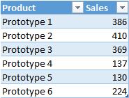
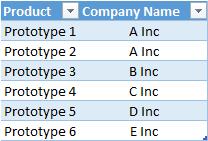
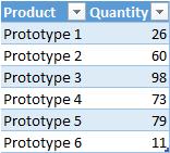
Consider we have three data tables, FactSales, CompanyTable and Product as shown below:

The data tables have a relationship mapping:

Table Product has a one-to-many relationship with table CompanyTable, which has a one-to-many relationship with table FactSales.

In table FactSales, we create two additional calculated columns, Product Quantity and Company respectively.  For Product Quantity, we use the LOOKUPVALUE function to look up the value for quantity based on the criteria product type:

The result column is in Product table, which represents the quantity we want to look up.  The search column is the product type in table Product and we set the criteria as the product type in table FactSales and the calculated column would be:

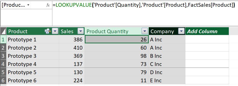
The column Product Quantity returns the quantity value stored in table Product by looking up to the same product type listed in FactSales.

Next step, we use the same logic to write the function for Company column with syntax below:

and the calculated column would be:

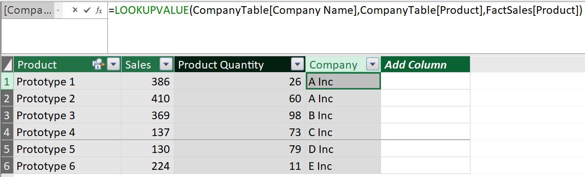
Column Company returns the company name by looking up the product type in table CompanyTable.

If we create a Pivot Table based on the relationship established by choosing the fields of Product, Company, the result would be:

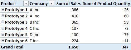
The Pivot Table above shows the company name, total sales and product quantity based on the product type.

That’s it for this week! Next week, we will apply the functions we have learned during the past few weeks to a business analytical scenario.

Stay tuned for our next post on Power Pivot in the Blog section. In the meantime, please remember we have training in Power Pivot which you can find out more about here. If you wish to catch up on past articles in the meantime, you can find all of our Past Power Pivot blogs here.