Monday Morning Mulling: October 2022 Challenge

On the final Friday of each month, we set an Excel / Power Pivot / Power Query / Power BI problem for you to puzzle over for the weekend.  On the Monday, we publish a solution.  If you think there is an alternative answer, feel free to email us.  We’ll feel free to ignore you.

The challenge this month was to find and replace multiple values at once in Excel. 

The Challenge

How did you usually find and replace a character in a text string in Excel?  Many people use the ‘Find & Replace’ functionality in Excel, which works fine for single replacements.  However, if you have tens, hundreds or thousands of items to replace this method seems very tedious and inefficient.  Luckily, there were several ways to do the mass replacement in Excel more elegantly and effectively.  Therefore, in this month’s challenge we challenged you to do that; you could download the question file here.

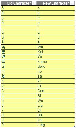
This month’s challenge was to write a formula to replace multiple letters in some text strings.  The replacement table (here, called Replace) might be as follows:

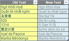
The result should look similar to the picture (below):

As always, there were some requirements:

• the formula needed to be within just one column (no “helper” cells)
• this was a formula challenge; no Power Query / Get & Transform or VBA
• the formula should be dynamic enough to update when a similar text string is added
• only Excel 2016 functions were accepted.

Suggested Solution

You can find our Excel file here which demonstrates our suggested solution.

Before we discuss the solution, I would like to note there are several complicating factors here.  Let’s go through them.

Problem 1: SUBSTITUTION – a Pragmatic Approach

For a standard approach, you might think of using multiple nested SUBSTITUTE functions here along with INDEX functions.  For example, if we have a single character to replace here, we will use the following formula:

In the formula above, the Texts, Replace is the name of the table.  Therefore, Texts[@Old Text], [@Old Character], and [@New Character] specify one row of column Text, Old Character, and New Character respectively.  If we want to replace two [2] characters, we can nest the function like this:

Therefore, with the same principle, if we want to replace n values, we will nest our function like this:

This pragmatic approach might work but it makes the function hard to inspect in case of any error occurs.  Besides that, it is not dynamic, if we put more characters to replace, we will have to modify the formula to adapt to the new inputs.  Therefore, this approach is rejected. 

Problem 2: Sequencing in the non-SEQUENCE world

When Dynamic Arrays were introduced, they introduced many useful Excel functions that come along with them, especially the SEQUENCE function.  This function helps us generate a list of sequential numbers in an array.  Hence, we can combine the SEQUENCE function with other functions like MID or LEN to transform the text string into individual cells in a spreadsheet with the following formula:

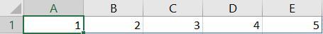
SEQUENCE(1, LEN(Texts[@Old Text])) will help us create a horizontal list of the consecutive text string from one [1] to the last number which is equal to the length of the string.  For example:

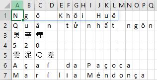
The MID function will then extract each character of a string with the starting point one by one, equal to the number list created by SEQUENCE above. 

However, the problem is SEQUENCE does not exist in Excel 2016.  Hence, we must find a workaround to do sequencing in “legacy” Excel that does not have the SEQUENCE function.  Rats.

Problem 3: Number or not Number?

One minor problem you might encounter is whether the value in the Replace table is in the number type or the text type.  Therefore, you have to convert these numbers into the same type.  If you do not convert them into the same type, it can cause a problem for you later on when you use any lookup or match function.  The idea here is that you also have to include the conversion within the formula as well.

Problem 4: Legacy Excel World

Before Dynamic Arrays became a thing, we had previously written an array formula in what we now call a legacy CTRL + SHIFT + ENTER (CSE) array.  Thus, what is the difference between those two? First, the “legacy” CSE array formulae require entering CTRL + SHIFT + ENTER after completing the formula.  For some formulae, we have to select a range for the output and then press the combination CTRL + SHIFT + ENTER whereas the Dynamic Array functions do not require this method of entry.  This is not an issue, but it requires us to visualise the outputs before they are generated so that we select the correct range for the outputs.

Brainstorming

To address the replacement for the SEQUENCE function, may we introduce you to the INDIRECT and ROW functions?  Let’s employ the following trick.  Consider the following formula:

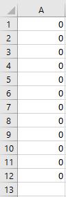
With respect to "A1:A"&LEN(Texts[@[Old Text]] this part of the formula will create a text string which is the range of the cell A1 to one of the cells in column A, depending upon the length of the text string.  For example, the first text string has 12 characters, so this piece of formula will return A1:A12.

Then we need a formula that can capture a text string here, since ROW requires a reference input, so it will not be able to capture a text reference here.  This is where the INDIRECT function comes in handy since it is used to capture the text reference.  Therefore, we wrap the INDIRECT around the text string above, then we will have the value of the first column.  However, it will return an #VALUE! error in some versions of Excel, so what you can do here is select the cell containing your formula and a range that equal to the length of the old text string you have.  Next, you press CTRL + SHIFT + ENTER, and voilà you generate the following:

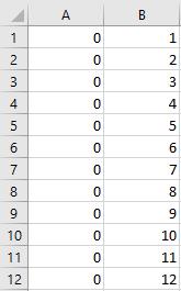
After that, we wrap the ROW function around the INDIRECT function we have.  Then, the formula we just create can mimic the SEQUENCE function which gives us the following sequence:

Backed to suggested solutions

Now return to the example of SEQUENCE, MID, and LEN functions we discuss in problem two [2], we can finally replace the SEQUENCE function with the formula we create earlier:

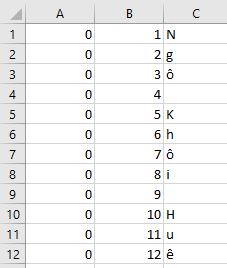
This formula will give us the following visual:

From here we can write a lookup function to match the character in the Texts[@[Old Text]] with the Replace[Old Character] and we return these matches with the accordance Replace[New Character]. 

Here we suggested you use the INDEX and MATCH functions.  We will have the following formula for the MATCH function:

This will be able to match correctly for the first second and third text strings but the fourth text string which is a number will not match.  This is the issue we discuss in problem three [3], so for it to work we must wrap our lookup array argument in the TEXT function to transform all the characters that have number type into text type.

Therefore, our complete function will look like this:

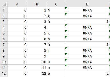
After writing the formula we will have the following visual:

Then we wrap the INDEX function around the MATCH function to replace the old characters in the text string with new characters:

So, we have the following array:

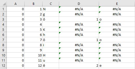
We need all the places where it shows #N/A! to keep the original text, so we can use the IFERROR function here:

Which will give us the following visual:

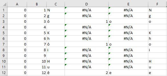
At this step, we introduced the last function that will help you merge all the arrays which is the CONCAT function.  The CONCAT function is the succeeding CONCATENATE function and is used to merge text.  Therefore, you wrap this function around all the formulas we have so far, and you will have the new text string here:

As we know CONCAT function will merge all our arrays into one [1] cell so, we can safely press CTRL + SHIFT + ENTER to get the results of multiple replacements.  Which will give you the following result table:

How cool is that?

Word to the Wise

Although this solution works quite well when replacing a single Replace[Old Character] in the Texts[@Old Text] for a single or multiple Replace[New Character], it cannot replace multiple characters of the Texts[@Old Text] with a single or multiple Replace[Old Character].  However, this could be a challenge for another Final Friday Fix…

The Final Friday Fix will return on Friday 25 November 2022 with a new Excel Challenge.  In the meantime, please look out for the Daily Excel Tip on our home page and watch out for a new blog every business working day.