A to Z of Excel Functions: The INDIRECT Function

Welcome back to our regular A to Z of Excel Functions blog.  Today we look at the INDIRECT function.

The INDIRECT function

Excel’s INDIRECT function allows the creation of a formula by referring to the contents of a cell, rather than the cell reference itself. 

The INDIRECT(ref_text,[a1]) function syntax has two arguments:

• ref_text: this is a required reference to a cell that contains an A1-style reference, an R1C1-style reference, a name defined as a reference or a reference to a cell as a text string.  If ref_text is not a valid cell reference, INDIRECT returns the #REF! error value.  If ref_text refers to another workbook (an external reference), the other workbook must be open.  If the source workbook is not open, INDIRECT again returns the #REF! error value.
• [a1] This is optional (hence the square brackets) and represents a logical value that specifies what type of reference is contained in the cell ref_text.  If a1 is TRUE or omitted, ref_text is interpreted as an A1-style reference.  If a1 is FALSE, ref_text is interpreted as an R1C1-style reference.  Most modellers seldom consider this alternative referencing approach, which is not without its merits (see below).

Essentially, INDIRECT works as follows:

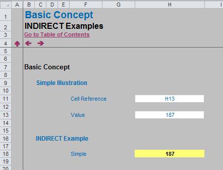
In the above example, the formula in cell H18 (the yellow cell) is

With only one argument in this function, INDIRECT assumes the A1-cell notation (e.g. the cell in the third row fourth column is cell D3).  Note that the value in cell H11 is H13, this formula returns the value / contents of cell H13, i.e. 187. 

This idea can be extended: the value indirectly referred to does not need to be in the same worksheet (or even workbook) as follows:

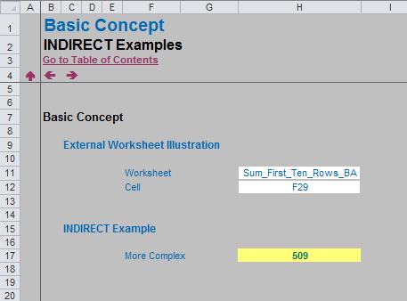
The formula in the yellow-coloured cell (H17) uses concatenation:

This formula is difficult to read.  Let’s make it clearer.  H11 in my example is Sum_First_Ten_Rows_BA, which is the name of another worksheet in the workbook and F29 is the cell to be linked to.  In other words, this formula becomes

which will make more sense to end users.  The point is, however, the value in cell H11 can be changed so that the formula suddenly links to a completely different worksheet.

Eagle-eyed readers may note that worksheet names without spaces do not need apostrophes.  Whilst this is true, I include them here so that the formula will work in general.

Advantages of INDIRECT

INDIRECT has useful properties that may be exploited.  For example, consider the following illustration:

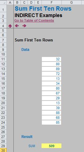
Imagine you wanted to sum the first ten values in this list.  The obvious formula to use would be

However, what happens if someone inadvertently inserts or removes rows in this range?  If a row were to be inserted the formula would automatically update to =SUM(F11:F21), which most of the time would be what would be required.  On occasion, though, it might be important that only the first ten values are still summed.  INDIRECT can ensure this happen, viz.

Note that when a reference is typed in like this it should be included in inverted commas as displayed.  Using this formula will maintain the integrity of the referencing as required.

So far, all of my examples use the A1-style of cell referencing.  However, using the R1C1 (row / column approach where the third row fourth column would be (3,4)) has benefits too.  When this method is used, I often use INDIRECT in conjunction with the ADDRESS function.

The

function syntax has the following arguments:

• row_number is a numeric value that specifies the row number to use in the cell reference
• column_number is also required and is a numeric value that specifies the column number to use in the cell reference.

Therefore =ADDRESS(3,4) is $D$3.

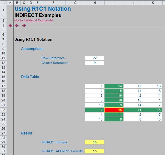
Just using INDIRECT in the example above, cell H29 uses concatenation once more:

The second argument (FALSE) is necessary to recognise the R1C1 notation.  Here, this formula reduces to =R22C9, which is the 22^nd row, ninth column, i.e. delivers the value in cell I22 (highlighted in red).

This formula can be difficult to understand for the uninitiated.  I am not saying the following is necessarily simpler, merely it is an alternative.  The second formula in cell H31 is

This does not need the R1C1 notation as ADDRESS(H11,H12) equals cell $I$22.

Another advantage I would like to mention is in generating dynamic data validation lists.  This example may be found in the attached Excel file:

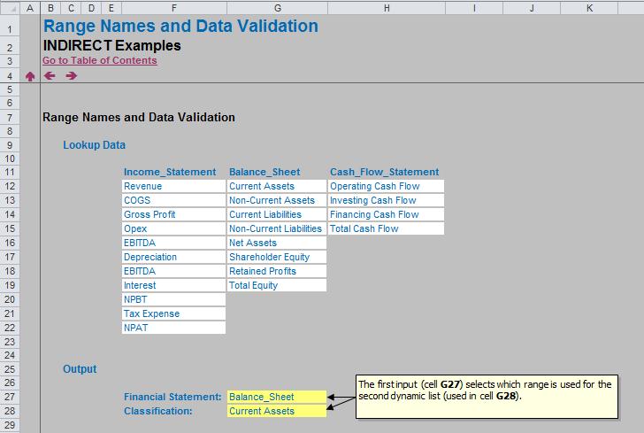
Here, I want to select a classification category in cell G28, based on the financial statement I select in cell G27 (e.g. Balance Sheet, Current Assets).

The trick here is not to include spaces in the names of the financial statements.

Then, first of all, in my illustration above, I have named cells F12:F22 Income_Statement, cells G12:G19 Balance Sheet and cells H12:H15 Cash_Flow_Statement. Cells F11:H11 have been used to construct a data validation list in cell G27 and then the data validation list in cell G28 has used the INDIRECT function in the ‘Source:’ field as follows:

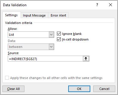
As a different financial statement is selected in cell G27, so the list will update in cell G28 (but only once the data validation list is activated, which is an Excel limitation).

One last – and key – example: how often do you seek a summary sheet which selects data from one of several similarly constructed datasheets?  I have seen all sorts of weird and wonderful formulae to perform this common requirement, but INDIRECT is by far one of the simplest approaches available.

Consider the following file, which has several similar worksheets:

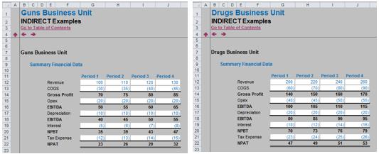
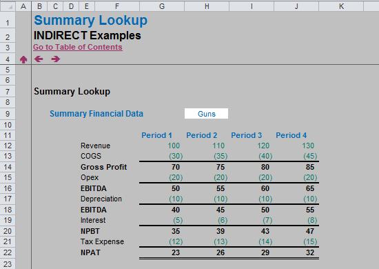
I might require a summary sheet:

In my example, I have called my similar worksheets Guns_BA and Drugs_BA.  The BA here refers to “Blank Assumptions” but it could mean “Basically Anything”, i.e. the worksheet names contain more than just the business unit name.

With cell H9 named Selection, the formula used in the calculations is simply

However, as well as apostrophes and concatenation this formula uses a neat trick.  The second argument must be FALSE (i.e. the formula assumes the R1C1 notation).  When this is selected the RC in the above formula means use the row and column reference of the cell this formula is in.  This avoids unnecessary hard code and generates a formula that changes reference depending upon the formula location in the worksheet.  For example, in cell G12, the formula reduces to =’Guns_BA’!G12 and in cell J21, it reduces to =’Guns_BA’!J21, etc.

Very useful!

Disadvantages of INDIRECT

Not all modellers embrace this useful function.  There are three key issues with INDIRECT:

1. INDIRECT encourages the use of hard code in formulae.  This should always be a last resort as this leads to a potential lack of transparency and flexibility in a model
2. INDIRECT is a difficult function to review / audit, as the cell(s) it refers to is not the ultimate location of the value used in the formula.  Excel’s in-built auditing tools are of limited use and the formulae can be highly confusing and ‘clunky’
3. If ref_text refers to a cell range outside the row limit of 1,048,576 or the column limit of 16,384 (XFD), INDIRECT returns an #REF! error.  However, this behaviour is different in earlier versions of Excel, which ignored the exceeded limit and returned an often meaningless value instead.  This can lead to compatibility issues between versions of Excel (admittedly, these earlier versions are outdated, no longer supported, and therefore, should not be used).

Ultimately, the use of INDIRECT becomes a subject “horses for courses” issue.  If modellers are knowledgeable and wary of its limitations, INDIRECT can simplify and resolve many common modelling problems.  Just be careful out there.

We’ll continue our A to Z of Excel Functions soon.  Keep checking back – there’s a new blog post every business day.

A full page of the function articles can be found here.