
Monday Morning Mulling: March 2025 Challenge
31 March 2025
On the final Friday of each month, we set an Excel / Power Pivot / Power Query / Power BI problem for you to puzzle over for the weekend. On the Monday, we publish a solution. If you think there is an alternative answer, feel free to email us. We’ll feel free to ignore you.
The Challenge
Last Friday’s challenge welcomed you to try and condense individual sets of values into a categorisation table with divisions A, B and C. As an example:
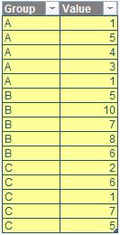
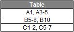
The table of individual sets (top) was provided, pairing a group classification with a corresponding value. A successful completion (bottom) would’ve entailed categorisation (A, B and C) of these values within their appropriate alphanumeric form.
How did this help you? By challenging you to strengthen your data condensing capabilities for all your storage, analysis and forecasting needs!
You could download the original question file here.
Remember, these were the requirements:
- the formula needed to be in just one cell (no “helper” cells)
- this was a formula challenge; no Power Query / Get & Transform or VBA!
Suggested Solution
You can find our Excel file here, which shows our suggested solution: you may have a better one. The steps are detailed below.
This process will find the alphanumeric solution for one group classification, group A, then provide the full formula configuration including all classifications. If you wish to skip right to the result you are more than welcome to do so.
Firstly, we need to find all unique groups so we may use its namesake, the UNIQUE function:
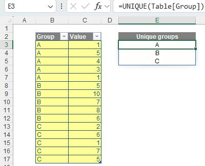
Performing this action would separate all unique groups into their appropriate rows. Since there were 3 different groups, A, B and C, you should see those listed.
Turning our focus to group A, we need to pull out its unique, associated numbers. We will utilise the UNIQUE function again, this time with the FILTER function which filters for only numbers associated with A, and the SORT function which will list those numbers in ascending order:
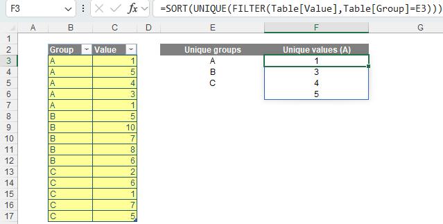
Since there are four [4] unique values associated with A, one [1], three [3], four [4] and five [5] in ascending order you should see those listed.
We now need to create a flag so Excel can determine where an alphanumeric code starts (and ends). To achieve this, we can use the logic that if a value is more than one [1] (in value) than the previous value, then that is the start of the next range:
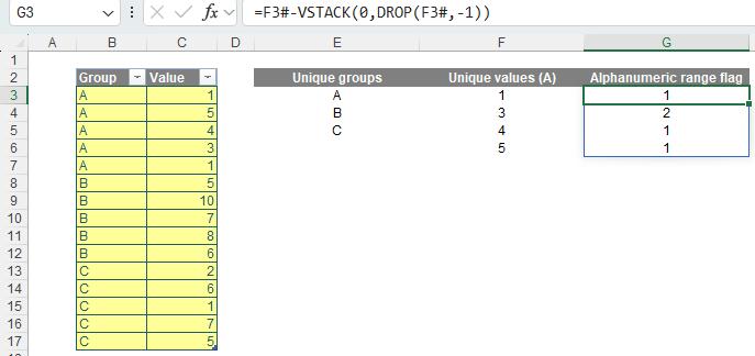
Therefore, we need to calculate changes in values. To get the predecessors, the values are shifted down as part of the VSTACK function with zero [0] as the starting value. The DROP function helps compensate for this shift down one [1] by cutting off the last row of the stack. Note that the VSTACK function is used to maintain the size of the spilled array.
A new alphanumeric code starts whenever the flag is higher than one so in this case, they will start at A1 and A3 (grouped values, not cell references!).
We now need to refine the flag so it returns group indices for the GROUPBY function:
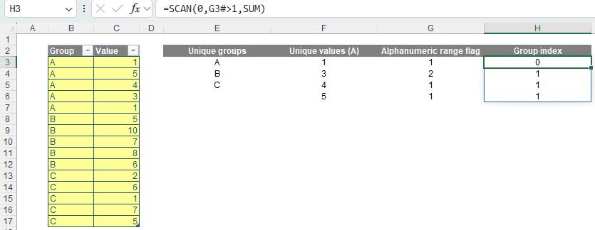
The SCAN function creates a rolling sum with an initial value of zero [0]. It identifies numbers greater than one [1], assigns a TRUE or FALSE value (one [1] or zero [0]) and then sums them. Since there is only one [1] value that satisfies the inequality, the rolling sum increases only at that point.
Next, this formula will be used:
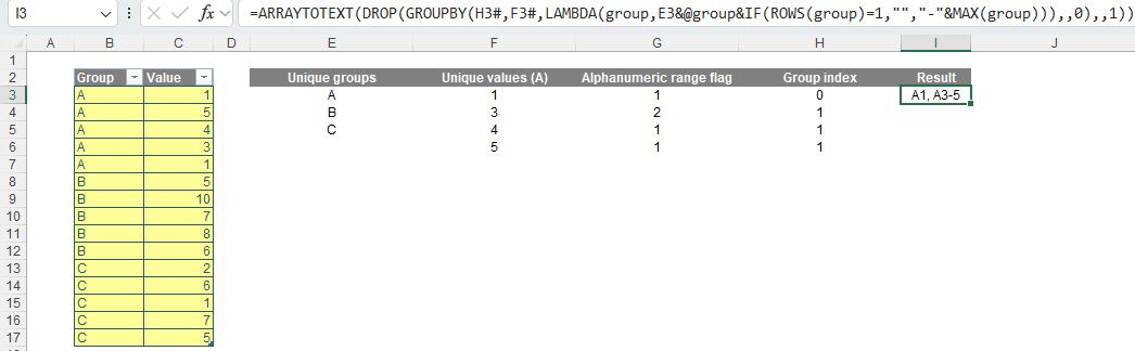
=ARRAYTOTEXT(DROP(GROUPBY(H4#,F4#,LAMBDA(group,
E4 & @group & IF(ROWS(group)=1, "",
"-"&MAX(group))),,0),,1))
The GROUPBY function groups all unique values (column F) by group index (column H) and summarises the grouped values based on the calculation in the LAMBDA function. It first concatenates group name (i.e. “A”) with the first value of each group using the @ symbol and an IF condition. If the number of rows of a group is not one [1] then it continues to concatenate with “-” and the maximum value of the group. As we don’t need to show the totals, zero [0] is specified in the 5th argument of GROUPBY. Then, the DROP function is used outside the GROUPBY to remove the first Group Index column. Finally, the resulting alphanumeric codes are combined together with a comma separator by the ARRAYTOTEXT function.
You should now see the alphanumeric form of all A classified values in alphanumeric form.
To arrive at the result that encompasses all classifications (A, B and C) and their associated values in alphanumeric form, you may use the combined formula:
=MAP(UNIQUE(Table[Group]), LAMBDA(type,
LET(value, SORT(UNIQUE(FILTER(Table[Value],Table[Group]=type))),
ARRAYTOTEXT(DROP(GROUPBY(
SCAN(0,value-VSTACK(0,DROP(value,-1))>1,SUM),
value,
LAMBDA(group, type & @group & IF(ROWS(group)=1, "",
"-"&MAX(group))),
,0
),,1)))))

A few things are added in this formula to account for the extra groups:
- the MAP function applies the mentioned calculations to each unique group and returns a transformed array
- the LET function allows us to name a variable to shorten the formula.
This will give:

How did you find it? It’s not the simplest concept we’ve ever discussed, that’s for sure. If you discovered an alternative approach, congratulations – that’s half the fun of Excel!
The Final Friday Fix will return on Friday 25 April 2025 with a new Excel Challenge. In the meantime, please look out for the Daily Excel Tip on our home page and watch out for a new blog every business working day.