Counting Unique Items in a List

When working with data, you often need to know how many unique items you have in a list.  For example, you might wish to know how many customers you have in your database, how many products you can offer to distributors or all the countries / geographical regions you make sales in.

The required data is frequently stored in tables or lists where duplication is rife.  Therefore, how do you “retire” the replicants without using Harrison Ford?  Today, I consider three non-lethal approaches reviewing the advantages and disadvantages of each.

First, let’s consider my data, highly tailored for the purposes of this article:

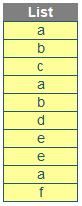
Or maybe not.

A cursory glance may glean the information you require: upon inspection, there are six unique items in the image, not including the heading (in case there are any smarty-pants out there).  But how do we get Excel to confirm this total?  I present three alternatives all detailed in the attached Excel file.

Option 1: Using Dynamic Arrays

Assuming the range (excluding the heading) is called Example1, I can employ the dynamic array formula UNIQUE.  That would be an obvious start, considering the title of this article.

Dynamic array formulae are calculations that use a function that will automatically extend its range depending upon the quantum of the results.  This automatic extending is known as spilling and although it potentially produces an array (a range of results that may encapsulate both more than one row and more than one column) it does not require to be entered using CTRL + SHIFT + ENTER, which is how array formulae needed to be entered in the past.

The hilarious thing about UNIQUE is that it does two things (!).  It details distinct items (i.e. provides each value that occurs with no repetition) and also it can return values which occur once and only once in a referred range.  It is the former feature we require here.

The UNIQUE function has the following syntax:

It has three arguments:

• array: this is required and represents the range or array from which to return unique values
• by_column: this argument is optional.  This is a logical value (TRUE / FALSE) indicating how to compare.  If you wish to compare by row, the argument should be FALSE or omitted (since this is the default).  To compare by column, you will need to select TRUE
• occurs_once:this argument is also optional.  This requires a logical value too:
  • TRUE: only return unique values that occur once
  • FALSE: include all distinct values (default if omitted).

It may sound complicated, but in truth, it isn’t.  Generating a unique list from Example1 is trivial:

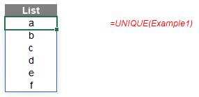
The formula

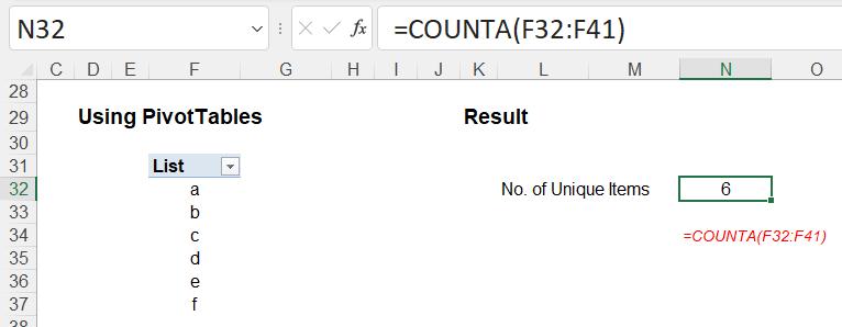
is both simple and intuitive to use, producing the list of the six [6] unique items in the order they are encountered (they are not sorted automatically – use the dynamic array function SORT to achieve this).  Once this has been derived, all we need to do is count the items in the list and COUNTA will achieve this as it counts the number of non-empty cells in a range:

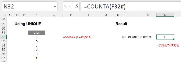
You should note that here the UNIQUE formula is in cell F32 and spills down the range F32:F37.  Highlighting this range will result in Excel displaying it as F32#, the hash / pound sign (#) denoting that the range may vary.  Therefore,

counts the spilled range emanating from cell F32 and hence totals the six [6] unique items.  You should note that blanks will appear as “0” in the range as will zeroes, but they will be treated as two different unique items, which is quite useful.

On this occasion, the formulae may be condensed (or “nested”):

Nesting array formulae does not always provide the required results due to the way Excel’s calculation engine works (this is discovered by using the universally and scientifically acclaimed approach known as “trial and error”!), but in this instance it will.

This method is remarkably simple and should be understood by the majority of Excel users.  However, it’s not all peaches and cream: dynamic arrays are only available in Excel 365 and Excel 2021 presently, so this is not available to all.  Call me old fashioned, but many get upset if they see #NAME? instead.  Therefore, this solution is useful only when all end users have dynamic array formulae at their disposal.

So what alternatives may we consider instead..?

Option 2: Using PivotTables

Everyone loves a good PivotTable, right..?  Firmly entrenched in the spreadsheeting software, there is no need to worry about version compatibility using a cross-tab query (what a delightfully scary name).

In this instance, I will first convert my source data into a Table (using Insert -> Table from the Ribbon or else the keyboard shortcut CTRL + T).  This allows the range to be automatically extended, without using those fancy dynamic array thingies (that’s a technical term, feel free to look it up).

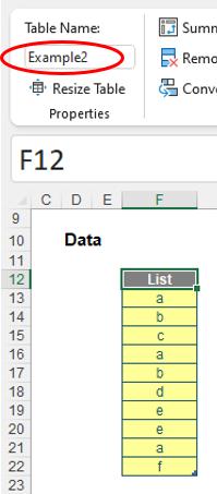
On the Ribbon, in the context-specific tab (i.e. when you select one or more cells of the Table) ‘Table Design’, you will note I have named this Table Example2. 

Next, I highlight one or more cells in this Table and select Insert -> PivotTable from the Ribbon (the keyboard shortcut varies depending upon the version of Excel you have, but typically starts ALT + N + V). 

I now view the ‘PivotTable Fields’ pane.  If it hasn’t shown up automatically, right-click in the resulting PivotTable and select the final option, ‘Show Field List’ (it’s annoying Excel refers to it as something else in the pop-up shortcut menu).  Then, simply move our only field (List) to the ‘Rows’ area, viz. 

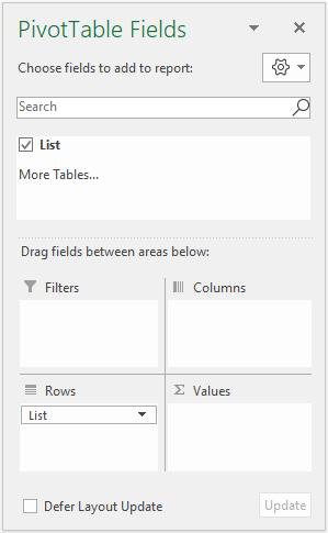
This produces the following PivotTable:

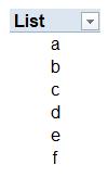
This list will be sorted alphanumerically by default.  Now, we simply count the number of non-blank items in this list.  If you had a blank item in your original list, don’t worry, it will still appear in the PivotTable as (blank) so will be treated as, er, non-blank.

There are a couple of drawbacks with this approach:

1. You should note that the COUNTA formula may need to include a larger range than is filled by the PivotTable.  This is in case the range extends when the data is refreshed.  This may cause issues if end users add other data to this worksheet.
2. If the source data changes, the PivotTable must be refreshed: the COUNTA formula will not necessarily provide the right answer until this action is performed.  Many users forget to do this.

Therefore, the idea is simple.  However, although it will work in all current versions of Excel, end users may forget to refresh the data should the source list be updated.  So what alternative do we have?

Option 3: Using SUMPRODUCT

Regular readers will know that SUMPRODUCT is one of my favourite functions in Excel, so much so that I named our company after it!  (It’s always good to get to Border Patrol and tell them I sell SUMPRODUCT for a living…)

The function is highly underestimated.  Consider the following example:

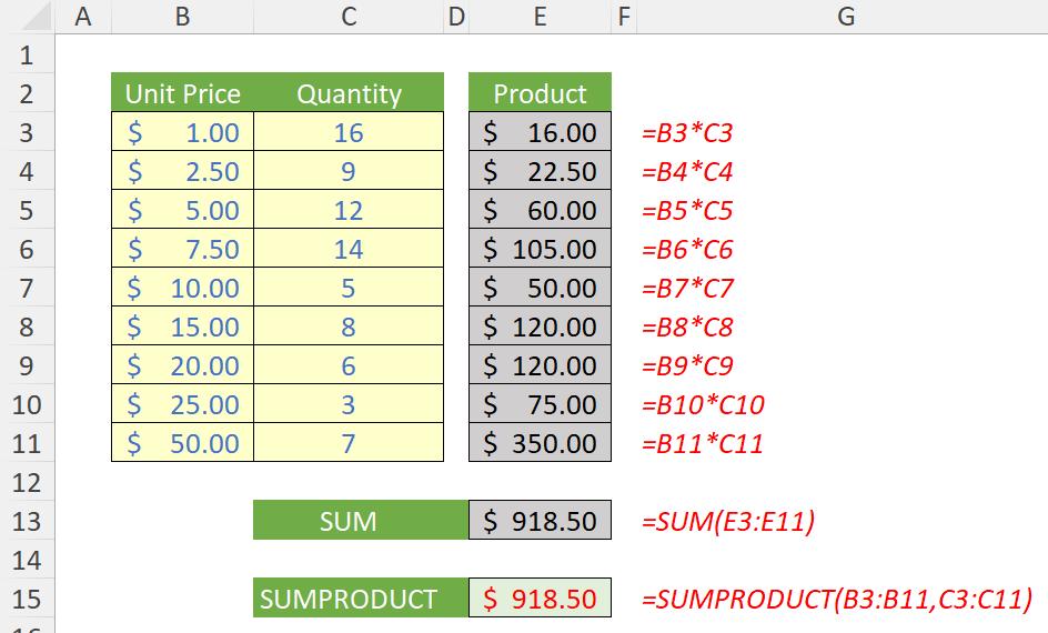
Here, I have various pricing points and the corresponding quantities sold.  To calculate my total sales, I can compute my sales by taking the product of Unit Price multiplied by Quantity on a line by line level and then summing them.  As you can see, SUMPRODUCT does it all in one go:

But SUMPRODUCT is more powerful than that.  The formula

does exactly the same thing.  Wow.  I bet that amazed you (not).  However, consider

Take a look at this revised example:

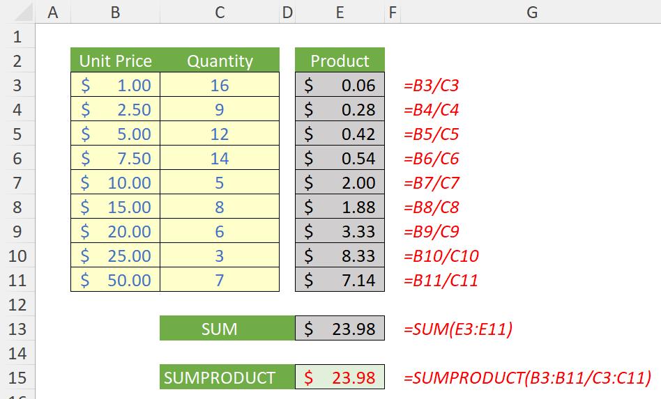
Do you see how SUMPRODUCT divides on a record by record basis?  This is powerful and it is this concept that I shall use for our final method to be employed today, using our list now conveniently called Example3:

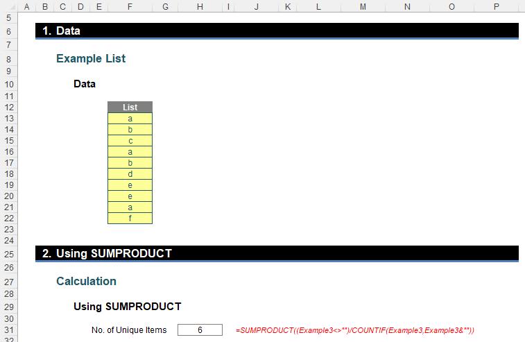
Here, I have used the formula

Clearly, this seems to work, although its logic may be a little less transparent that than the other two approaches upon first glance.  The initial condition

checks whether the range Example3 contains non-empty cells (TRUE if so, FALSE otherwise).  Here, it does not need to be non-blank – it just needs to be anything that cannot occur in the list in this scenario.  You could just substitute this for one [1] should you wish, but I wanted to demonstrate how this might work if you wished to exclude blank cells.  This gives us

The second part,

uses one of the more unusual ways of using COUNTIF.  Again it returns an array, but this time each value in the array represents a count of the numbers in the array using each value of the array as a criterion (the &“” addendum merely coerces the value to a text string, which may be required in certain instances).  This results in

i.e. there are three [3] instances of “a”, two [2] of “b” and so on.  The numerator is then divided by the denominator on an item by item basis to give us

When used in mathematical operations, TRUE behaves like one [1] and FALSE behaves as if it were zero [0].  These results are then summed together to give us six [6].  Easy when you know how.

The advantage of this approach is that it neither requires dynamic arrays nor data refreshing.  The problem is the calculation is a little opaque, but hey, “Obfuscate” is my middle name.  No solution is perfect, but this final option may prove to be the best all-rounder.

Word to the Wise

Some of you may be surprised that I did not use Power Query / Get & Transform as one of the options above, since removing duplicates is a base transformation in the Power Query Editor.  For the arbitrary purposes of this article, I merely wanted to consider basic Excel features and functions.

Indeed, Get & Transform may be used too.  It is a great method for cleansing data where there may be surplus spaces (trimming), non-printable characters (cleaning) or a preponderance of haphazard upper / lower case lettering.  However, similar to the PivotTables solution detailed above, this requires data to be refreshed in order to be updated, which many end users forget.  Therefore, given the “behind the scenes” nature of this option, I chose to discount it in this instance.  Nonetheless, this extract / transform / load (ETL) tool should be viewed as an essential tool in every modeller’s armoury.  It’s merely a case of knowing which may work best when.