
A to Z of Excel Functions: The FILTER Function
24 May 2019
Welcome back to our regular A to Z of Excel Functions blog. Today we look at the FILTER function.
The FILTER function
Still in what Microsoft refers as “Preview” mode, i.e. it’s not yet “Generally Available”, FILTER is one of seven functions heralding the new dawn of arrays – the Dynamic Array. Presently, you need to be part of what is called the “Office Insider” programme which is an Office 365 fast track. You can register in File -> Account -> Office Insider in Excel’s backstage area.
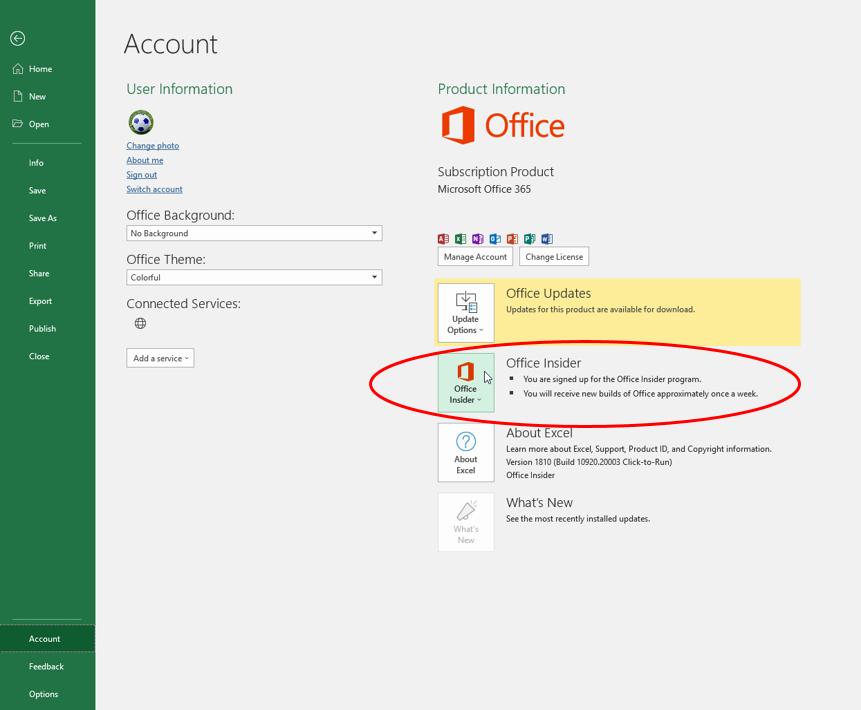
Even then, you’re not guaranteed a ticket to the ball as only some will receive the new features as Microsoft slowly roll out these features and functions. Please don’t let that put you off. These features and this function will be with all Office 365 subscribers soon.
Before explaining FILTER, let’s first consider what a Dynamic Array is. Consider the following data:
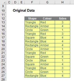
If I were to type =F12:H27 into another cell, Excel in the past would have thought I had gone mad. I’d need to wrap it in an aggregation function such as SUM, COUNT or MAX, to name but a few. Otherwise, I would have to wrap it in braces using CTRL + SHIFT + ENTER and use it as an array formula.
But no more.
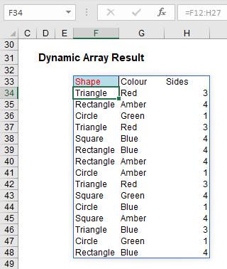
Look at what happens when I type =F12:H27 into cell F33:
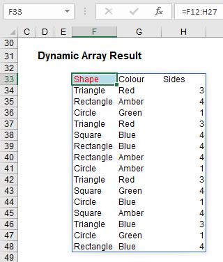
The formula automatically extends to three columns by 16 rows! It has spilled. Get used to the vernacular. There’s a reason this article got the name it did!
Any formula that has the potential to return multiple results can be referred to as a Dynamic Array formula. Formulae that are currently returning multiple results, and are successfully spilling, can be referred to as Spilled Array Formulae.
Notice I did not have to highlight all of the cells F33:H48. It spilled. Also take note I formatted cell F33 – er, that didn’t spill, because presently formatting isn’t propagated. This is why this is not yet Generally Available. Microsoft is still trying to work out what should and shouldn’t be allowed to happen in this first release. But don’t let that put you off.
And don’t let this basic example put you off either. If you feel a general sense of underwhelm coming over you, it’s because I haven’t yet communicated how powerful this all is as my example was too basic.
However, before I carry on there is a question I do need to cover with my far too simple example: what happens if something gets in the way?
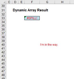
In this example, in cell G40, I have typed in the obtrusive text, “I’m in the way”. And it quite literally is. Consequently, I have generated the brand new #SPILL! error. The formula cannot spill, so the error message is generated accordingly.
#SPILL! Errors
#SPILL! errors are returned when a formula returns multiple results, and Excel cannot return the results to the spreadsheet. There are various reasons an #SPILL! error could occur:
- spill range is not blank: as in my example (above), this error occurs when one or more cells in the designated spill range are not blank and thus may not be populated.
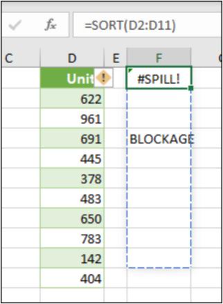
- When the formula is selected, a dashed border will indicate the intended spill range. You may select the error “floatie” (believe it or not, this is what Microsoft call these things!), and choose the ‘Select Obstructing Cell’ option to immediately go the obstructing cell. You can then clear the error by either deleting or moving the obstructing cell's entry. As soon as the obstruction is cleared, the array formula will spill as intended
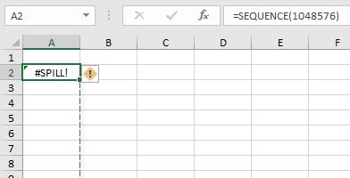
- the range is volatile in size: this means the size is not “set” and can vary. Excel was unable to determine the size of the spilled array because it's volatile and resizes between calculation passes. For example, the new function SEQUENCE(x) generates a list of x numbers increasing by 1 from 1 to x. That’s fine, but the following formula will trigger this #SPILL! error:
=SEQUENCE(RANDBETWEEN(1,1000)).
- Dynamic array resizes may trigger additional calculation passes to ensure the spreadsheet is fully calculated. If the size of the array continues to change during these additional passes and does not stabilise, Excel will resolve the dynamic array as #SPILL! This error type is generally associated with the use of RAND, RANDARRAY and RANDBETWEEN functions. Other volatile functions such as OFFSET, INDIRECT and TODAY do not return different values on every calculation pass so tend not to generate this error
- extends beyond the worksheet’s edge: in this situation, the spilled array formula you are attempting to enter will extend beyond the worksheet's range. You should try again with a smaller range or array. For example, moving the following formula to cell A1 will resolve the error, and the formula will spill correctly
- Table formula: as I will explain shortly, Tables and Dynamic Arrays are not yet best friends. Spilled array formulae aren't supported in Excel Tables (generated by CTRL + T). Try moving your formula out of the Table, or go to Table Tools -> Convert to range
- out of memory: I have forgotten what this one means. Sorry, I couldn’t resist that. The spilled array formula you are attempting to enter has caused Excel to run out of memory. You should try referencing a smaller array or range
- spill into merged cells: spilled array formulae cannot spill into merged cells. You will need to un-merge the cells in question or else move the formula to another range that doesn't intersect with merged cell
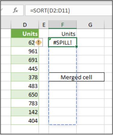
- When the formula is selected, a dashed border will indicate the intended spill range. You can again select that wonderfully named error floatie and choose the ‘Select Obstructing Cell’ option to immediately go the obstructing cell. As soon as the merged cells are cleared, the array formula will spill as intended
- unrecognised / fallback error: the “catch all” variant. Excel doesn't recognise, or cannot reconcile, the cause of this error. Here, you should make sure your formula contains all of the required arguments for your scenario.
Returning to Dynamic Arrays
Now that we have considered what happens if you block a Dynamic Array, let me now turn my attention to what happens if you don’t. You get the following:
Do you see I am not having to anchor cells (i.e. use dollar [$] signs)? The formula just spills. Let me be clear. If I select cell F34, I get the following:
Here’s a first. Check out the formula in the formula bar. It’s greyed out. Ever seen that before? Effectively, cell F34 contains the value ‘Triangle’ but it does not actually contain an “Excel” formula in the usual sense. To demonstrate this, let me show you the VBA Immediate Window:
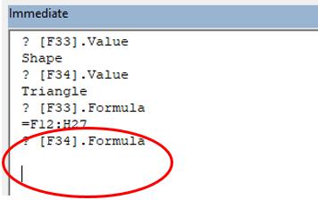
If you select cells F33:H48 and use ‘Go To Special’ (F5 -> Special), and then select ‘Formulas’, cells F33:H48 are shown as formula cells. You can even copy and paste them as values. Ladies and gentlemen, welcome to this brave new world.
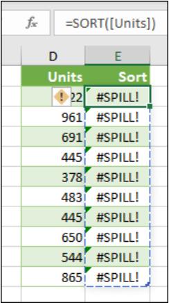
Once you have a Dynamic Array, referring to it is simple using what is known as the Spilled Range Operator. For example, if I want to refer to the Dynamic Array in the previous examples, it initially had a range of L57:N72. However, once I had added a row and column to the Table, this resized to L57:O73. I can easily refer to this array, whatever its size as follows. In its initial state:
The formula =L57# allows for variations – you simply type in the top left-hand cell reference (i.e. the cell with the non-greyed out formula) and add "#”, known as the Spilled Range Operator. Simple!
FILTER Function
With the above borne in mind, the FILTER function will accept an array, allow you to filter a range of data based upon criteria you define and return the results to a spill range.
The syntax of FILTER is as follows:
=FILTER(array, include, [if_empty]).
It has three arguments:
- array: this is required and represents the range that is to be filtered
- include: this is also required. This specifies the condition(s) that must be met
- if_empty: this argument is optional. This is what will be returned if no data meets the criterion / criteria specified in the include argument. It’s generally a good idea to at least use “” here.
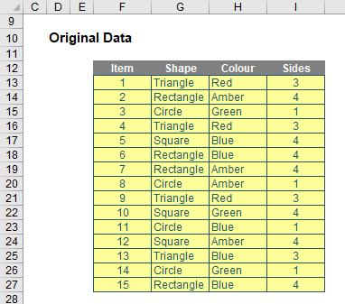
For example, consider the following source data:
To begin with, I will perform a simple FILTER:
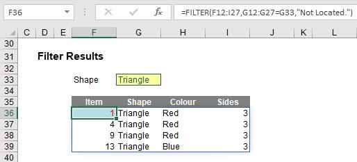
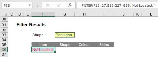
Here, in cell F36, I have created the formula
=FILTER(F12:I27,G12:G27=G33,”Not Located.”)
F12:I27 is my source array and I wish only to include shapes (column G12:G27) that are ‘Triangles’ (specified by cell G33). If there are no such shapes, then “Not Located.” is returned instead. To show this, I will change the shape as follows:
That is about as basic as it gets. I can get cleverer. Consider the following example:
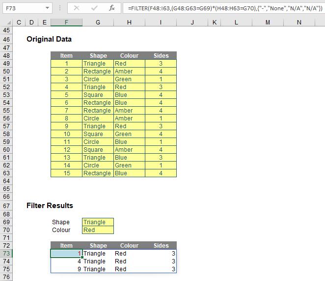
I have repeated the source array (cells F48:I63) for clarity. The formula
=FILTER(F48:I63,(G48:G63=G69)*(H48:H63=G70),{"-","None","N/A","N/A"})
looks horrible to begin with, but it’s not quite as bad as it appears upon further scrutiny. The include argument,
(G48:G63=G69)*(H48:H63=G70)
contains two conditions. Firstly, G48:G63=G69 means that the ‘Shape’ (column G48:G63) has to be a ‘Triangle’ (cell G69) and that the ‘Colour’ (column H48:H63) has to be ‘Red’ (cell G70). The multiplication operator (*) is used to denote AND. The Excel function AND cannot be used with arrays – this is nothing special to Dynamic Arrays; AND does not work with CTRL + SHIFT + ENTER formulae either. This syntax is similar to how you would create AND criteria with the SUMPRODUCT function, for example.
Consider the final argiment: {"-","None","N/A","N/A"}. The braces (typed in!) are used to create an array argument that specifies what should be written in each column should there be no record that meets both criteria, e.g.
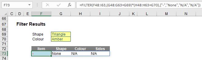
See? Not as bad as you might first think.
My final example is very similar:
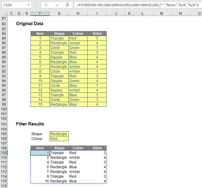
Once you realise I have simply repeated referencing for clarity, the formula
=FILTER(F84:I99,(G84:G99=G105)+(H84:H99=G106),{"-","None","N/A","N/A"})
is nothing more than the OR equivalent of the previous example, with ‘+’ replacing ‘*’ to switch from ensuring both conditions are met to only one condition being met. As at the time of writing, XOR is not catered for, but I am sure some clever person will create an equivalent in due course (if Microsoft doesn’t beat them to it), necessity being the mother of invention and all that jazz.
Dynamic Arrays vs. Legacy Array Formulae
Finally, prior to this new functionality, if you wanted to work with ranges in Excel, you used to have to build array formulae, where references would refer to ranges and be entered as CTRL + SHIFT + ENTER formulae. The main differences are as follows:
- Dynamic Array formulae may spill outside the cell bounds where the formula is entered. The Dynamic Array formula technically only exists in the cell in the top left-hand corner of the spilled range (as shown earlier), whereas with a legacy CTRL + SHIFT + ENTER formula, the formula would need to be entered in the entire range
- Dynamic arrays will automatically resize as data is added or removed from the source range. CTRL + SHIFT + ENTER array formulae will truncate the return area if it's too small, or return #N/A errors if too large
- Dynamic array formulae will calculate in a 1 x 1 context
- Any new formulae that return more than one result will automatically spill. There's simply no need to press CTRL + SHIFT + ENTER
- According to Microsoft, CTRL + SHIFT + ENTER array formulae are only retained for backwards compatibility reasons. Going forward, you should use Dynamic Array formulae instead
- Dynamic array formulae may be easily modified by changing the source cell, whereas CTRL + SHIFT + ENTER array formulae require that the entire range be edited simultaneously
- Column and row insertion / deletion is prohibited in an active CRL + SHIFT + ENTER array formula range. You first need to delete any existing array formulas that are in the way.
We’ll continue our A to Z of Excel Functions soon. Keep checking back – there’s a new blog post every business day.
A full page of the function articles can be found here.