
Monday Morning Mulling: January 2023 Challenge
30 January 2023
On the final Friday of each month, we set an Excel / Power Pivot / Power Query / Power BI problem for you to puzzle over for the weekend. On the Monday, we publish a solution. If you think there is an alternative answer, feel free to email us. We’ll feel free to ignore you.
The challenge this month was to replicate a Table, removing entries containing specified values using a formula in Excel.
The Challenge
Filtering data in a Table in Excel is as easy as clicking the filter button then ticking the data you want, right? However, if you want to see all but a few choice options in a field with many different entries, you may find yourself scrolling tirelessly to find and untick the few you don’t want to see. Luckily, there are several ways to filter data based off of a list of values to exclude, which can be achieved using only formulae. In this month’s challenge, we invited you to do just that; you could download the question file here.
This month’s challenge was to write a formula to replicate data in a Table, removing entries as specified in a second Table. The starting Table (here, imaginatively called Data) might be as follows:

The data to remove Table (named Remove) may look like this:

The result, using the inputs shown, should have looked similar to the below:

As always, there were some requirements:
- the formula needed to be within just one cell (no “helper” cells)
- this was a formula challenge; no Power Query / Get & Transform or VBA
- the formula should have been dynamic enough to update when entries were added to the Remove Table.
Suggested Solution
You can find our Excel file here which demonstrates our suggested solution.
Before we begin, let’s discuss the three functions we’ve used in conjunction to construct our solution.
The FILTER Function
You can read our full article on the FILTER function here. FILTER is one of Excel’s Dynamic Array formulae. It will accept an array and allow you to filter this based upon criteria you define, returning the results to a spilled range.
The syntax of FILTER is as follows:
=FILTER(array, include, [if_empty])
It has three arguments:
- array: this is required and represents the range that is to be filtered
- include: this is also required. This specifies the condition(s) that must be met
- if_empty: this argument is optional. This is what will be returned if no data meets the criterion / criteria specified in the include argument. It’s generally a good idea to at least use “” here.
The include argument must evaluate to an array made up of true or false and be either the same height or width as the array.
The MATCH Function
You can read our full article on the MATCH function here. The MATCH function will return the relative position of an item in an array that (approximately) matches a specified value.
The syntax is as follows:
=MATCH(lookup_value, lookup_vector, [match_type])
It has three arguments:
- lookup_value: this is required and is the value that you want to match in lookup_array
- lookup_vector: this is required and is the range of cells being searched
- match_type: this is optional and can be either -1, 0 or 1. This specifies how Excel matches lookup_value with values in lookup_vector. The default argument is one [1].
The different type of match are as follows:
- match_type 1 [default if omitted]: finds the largest value less than or equal to the lookup_value – but the lookup_vector must be in strict ascending order, limiting flexibility
- match_type 0: probably the most useful setting, MATCH will find the position of the first value that matches lookup_value exactly. The lookup_array can have data in any order and even allows duplicates
- match_type -1: finds the smallest value greater than or equal to the lookup_value – but the lookup_vector must be in strict descending order, again limiting flexibility.
When using MATCH, if there is no (approximate) match, #N/A is returned (this may also occur if data is not correctly sorted depending upon match_type).
The ISERROR Function
You can read our full article on the ISERROR function here. This function checks whether the value is an error and returns either TRUE or FALSE accordingly.
The syntax is as follows:
ISERROR(value)
It has only one argument:
- value: this is required and represents the value you want to test
Our Solution
Understanding those three functions, we can take a look at our solution:
=FILTER(Data,ISERROR(MATCH(Data[Item],Remove[Remove],0)),{"N/A","-","-","-"})
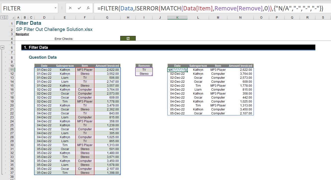
We have chosen to use the FILTER function on our table (named Data), keeping only values where the following argument evaluates to true:
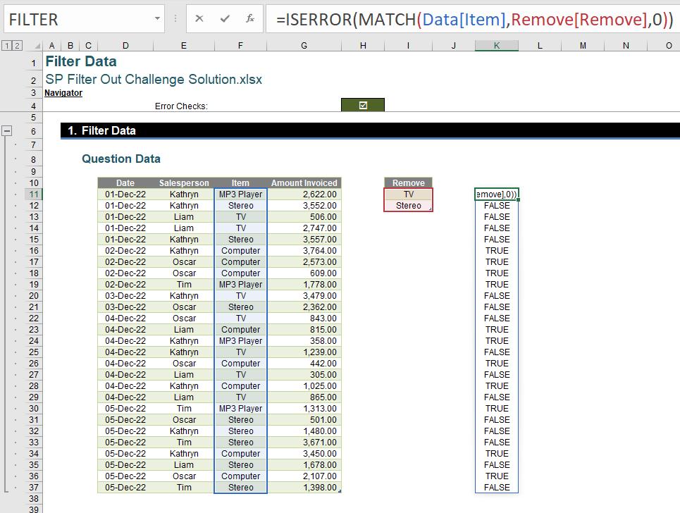
ISERROR(MATCH(Data[Item],Remove[Remove],0))
Working backwards through this argument, we first use the MATCH function (with the third argument set to 0, looking for an exact match) to attempt to match each entry in the Item field in our Data table to an entry in the Remove table. This will return a number for each row where the Item field contains a value in our Remove table and an error (#N/A) for rows that do not contain one of these values.

As we wish to keep rows that do not contain values in the Remove table, we will want our errors to evaluate to TRUE and our numbers to evaluate to FALSE; we have achieved this using the ISERROR function.
Finally, looking at the third argument of our FILTER function:
{"N/A","-","-","-"}
This is telling our function what to output if the filtered range is empty (i.e. no data meets the criteria / criterion), ensuring that our function will not result in an error even if all unique entries in the Item field are included within the Remove table.

But what if we wanted to filter out values in multiple columns? Well, that’s one for another time…
The Final Friday Fix will return on Friday 24 February 2023 with a new Excel Challenge. In the meantime, please look out for the Daily Excel Tip on our home page and watch out for a new blog every business working day.