Monday Morning Mulling: April 2023 Challenge

On the final Friday of each month, we set an Excel / Power Pivot / Power Query / Power BI problem for you to puzzle over for the weekend.  On the Monday, we publish a solution.  If you think there is an alternative answer, feel free to email us.  We’ll feel free to ignore you.

The challenge this month was to extract data and add it to the Table.  Did you succeed?

The Challenge

This month, we had a Power Query challenge. 

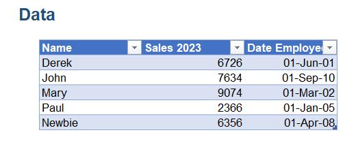
We provided a challenge file which includes the following Table of data for our imaginary tent salespeople:

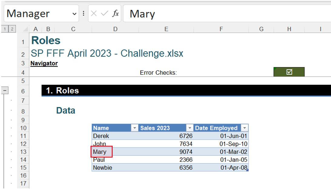
One of our esteemed salespeople has been promoted to be the manager of the team.  This information appears in a Named Range pointing at cell $D$13:

You can download the challenge file here.

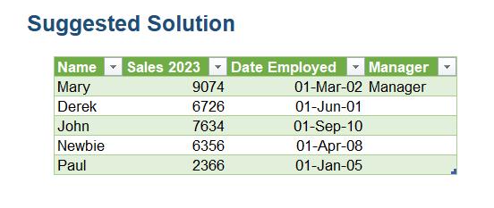
This month’s challenge was to combine the Table with the information in the Named Range, and present it in a new Table:

As always, there were some conditions:

• This is a Power Query challenge - No Excel formulae allowed!
• No hard-coding should be used to determine the contents or the name of column Manager.

Suggested Solution

You can find our Excel file here which demonstrates our suggested solution.

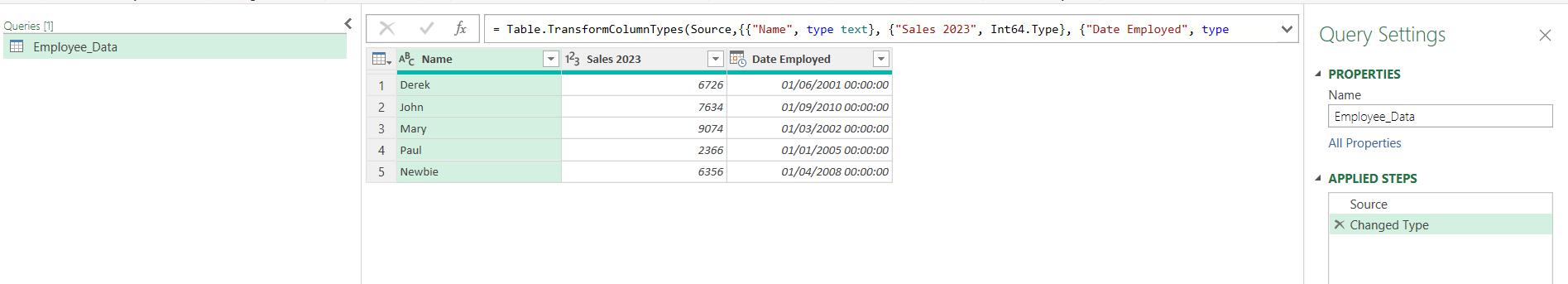
We start by extracting the data.  We can select the data and choose ‘From Table/Range’ in the ‘Get & Transform Data’ section of the Data tab.  

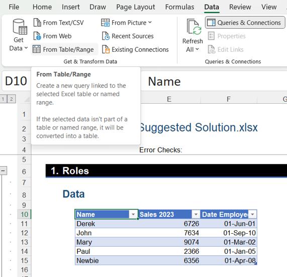
This gives us a query for the Table Employee_Data:

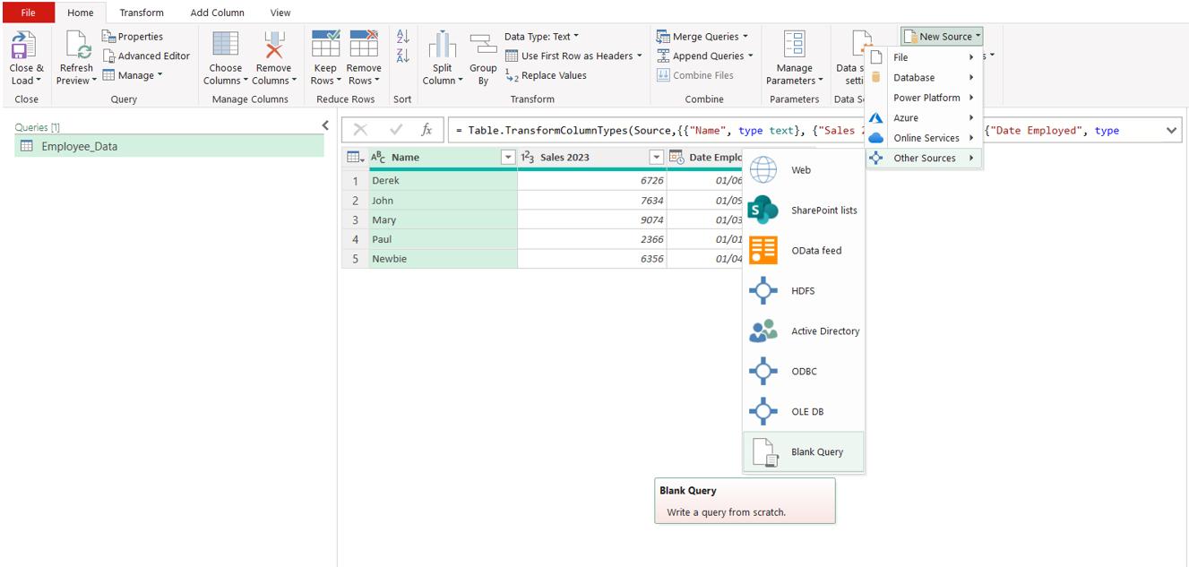
Next, we create a new Blank Query:

We call this query Workbook_Data, and enter some simple M code to get started:

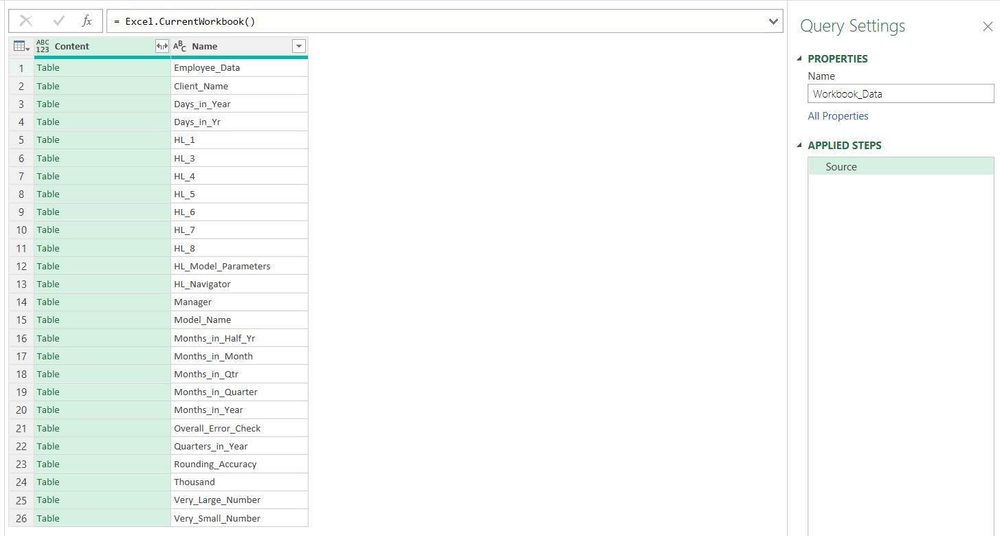
The M code we have entered is:

This gives us the contents of the Excel workbook.  We need to expand the Tables in the Content column.

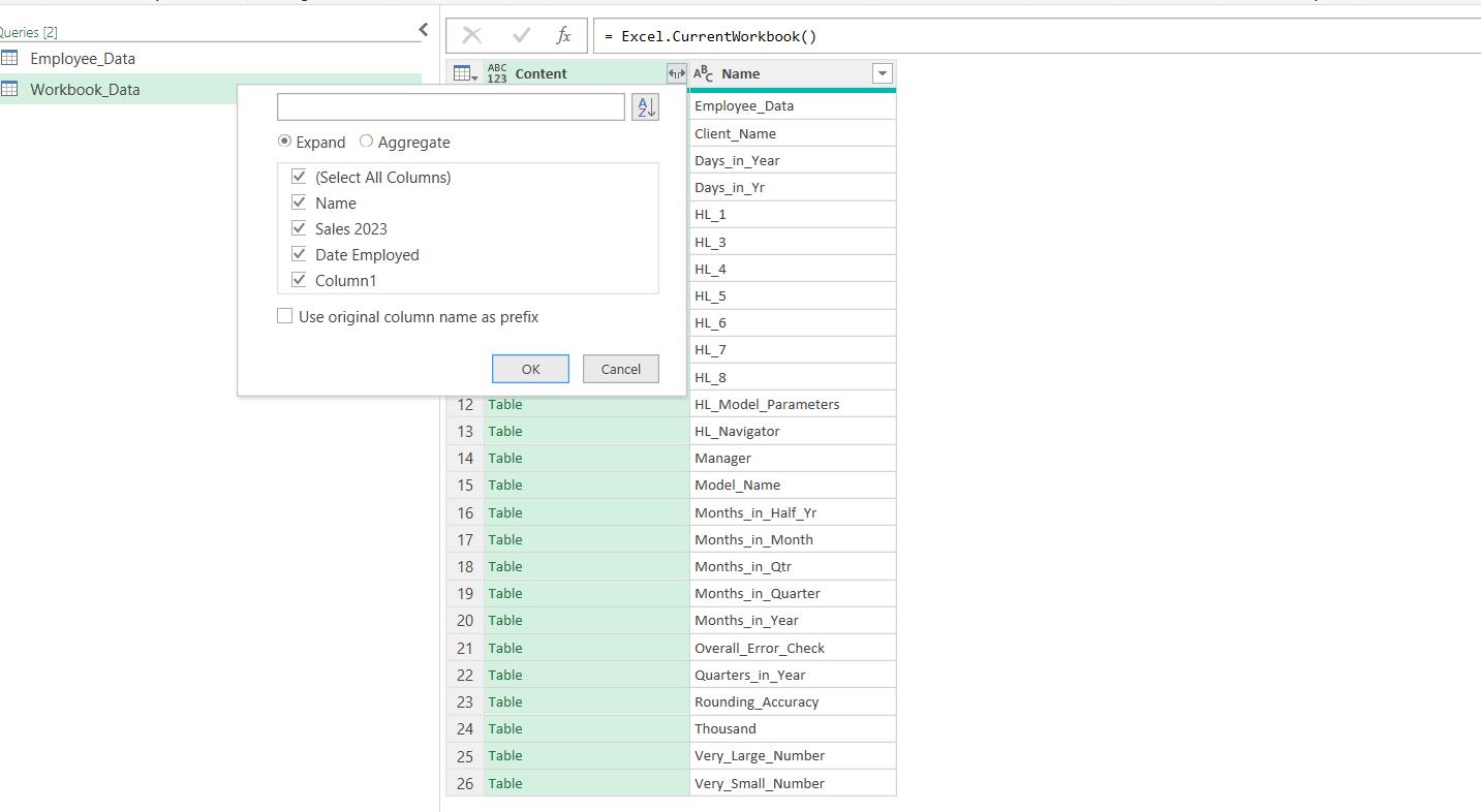
We uncheck ‘Use original column name as prefix’, and click ‘OK’ to see the data:

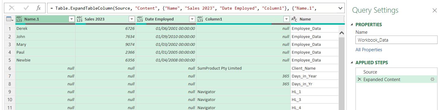
We can see that the first three columns are from the Employee_Data table, so we can select them, and press delete to remove them.

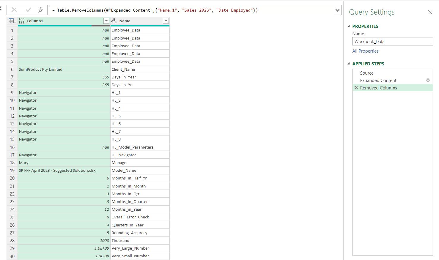
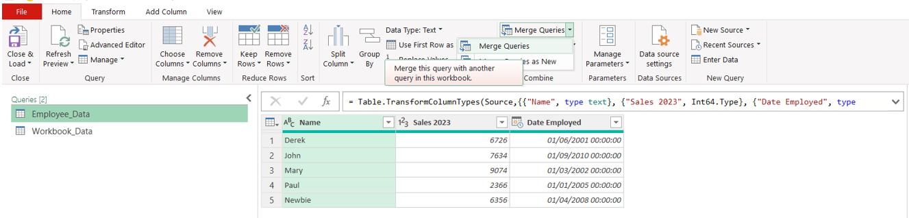
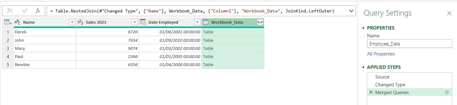
We can see that Column1 contains the target of Defined Names in Excel.  We can go back to the Employee_Data query and ‘Merge Queries’ from the Home tab:

We merge with Workbook_Data, looking for any connections to our salespeople:

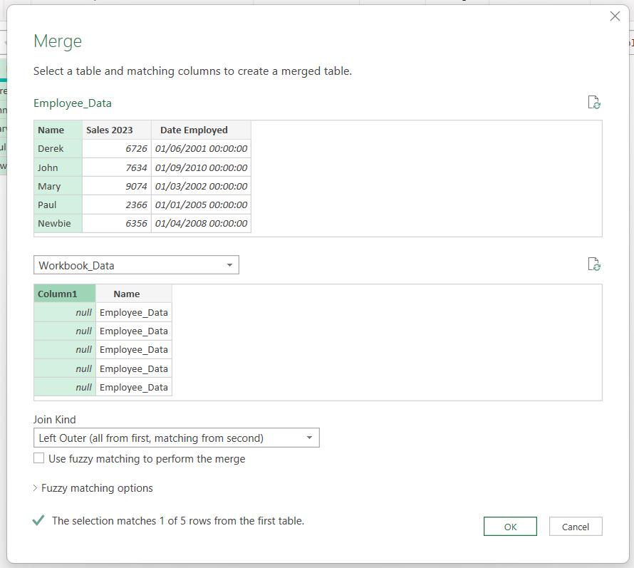
We can see that one [1] employee has a match, so we click OK to continue.

We need to expand the data, but we only need one [1] column:

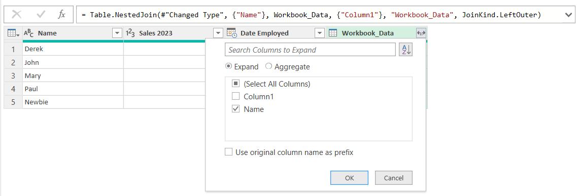
This gives us the information we need.

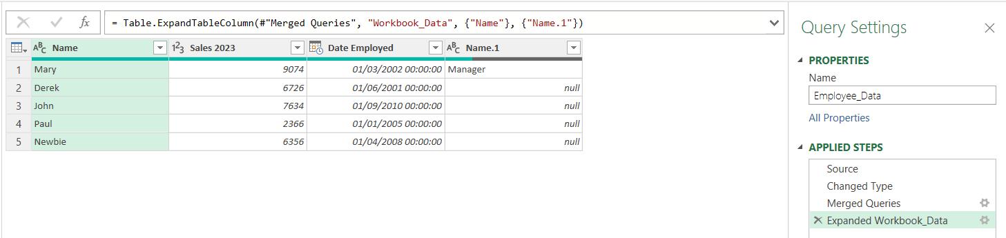
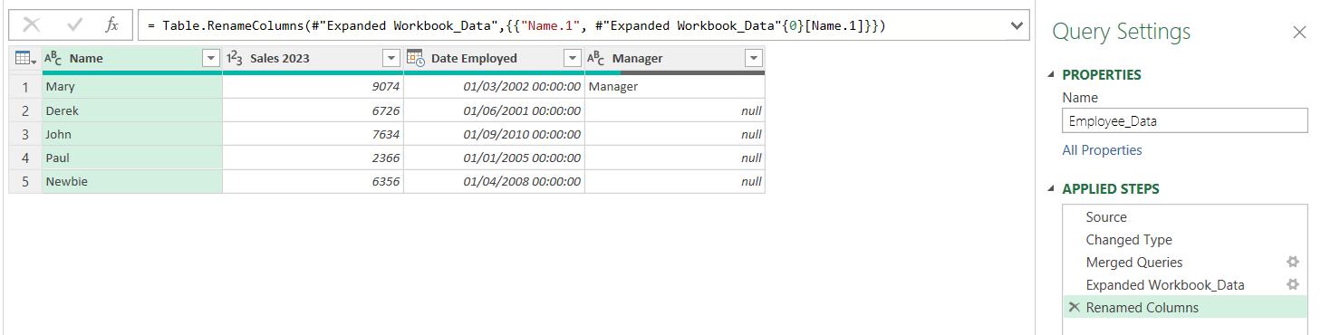
Now we need to rename the Name.1 column to Manager, so we begin by creating the step:

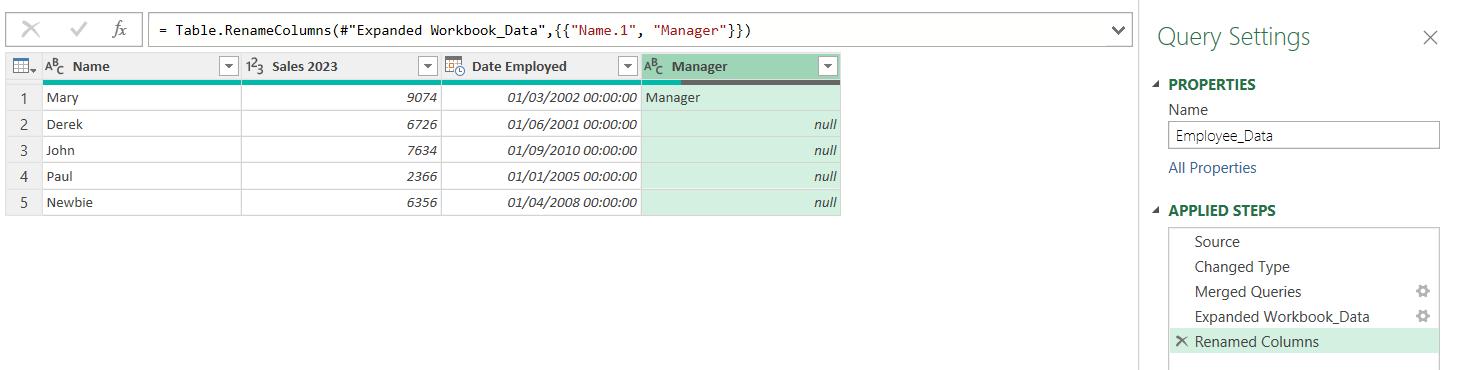
However, we need to do this with no hard-coding, so we are going to replace the current M code:

with this:

This extracts the name from the first instance of column Name.1 in the previous step.

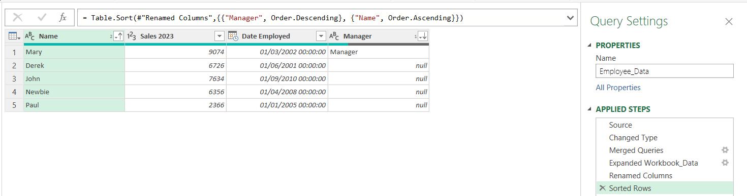
We sort on Manager in descending order, and then Name in ascending order, which Power Query combines into one step:

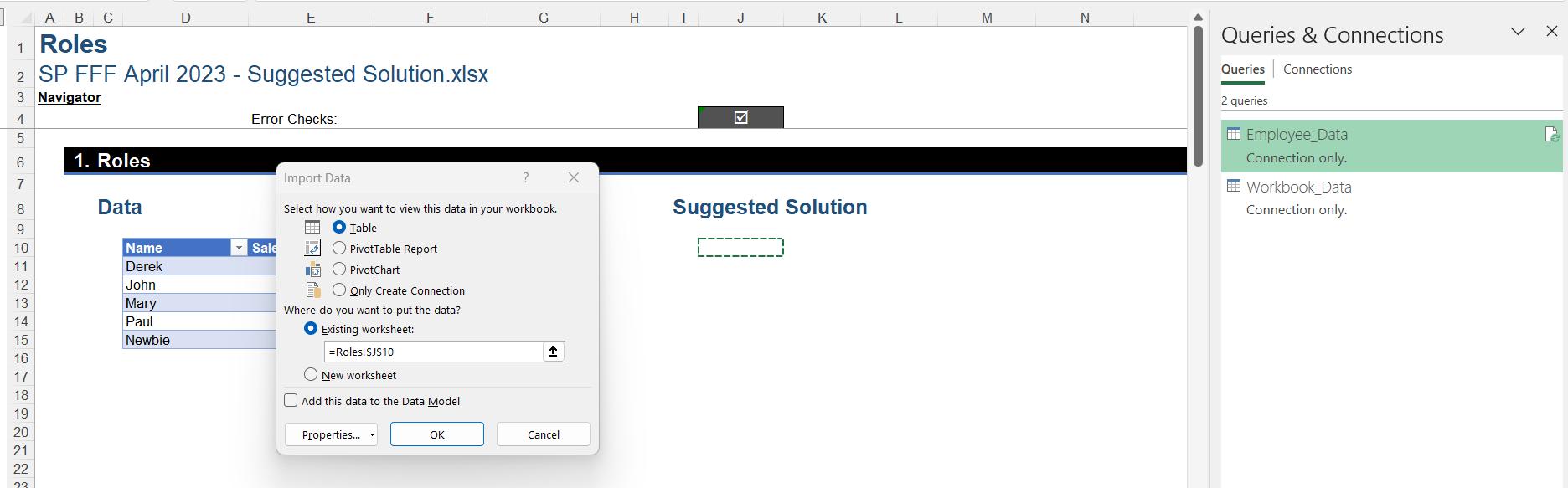
We choose to ‘Close & Load To…’ from the Home tab and initially set both queries to ‘Connection only’.  We can then right-click on the Employee_Data query and choose to load to ‘Table’ and place it on the ‘Existing worksheet’:

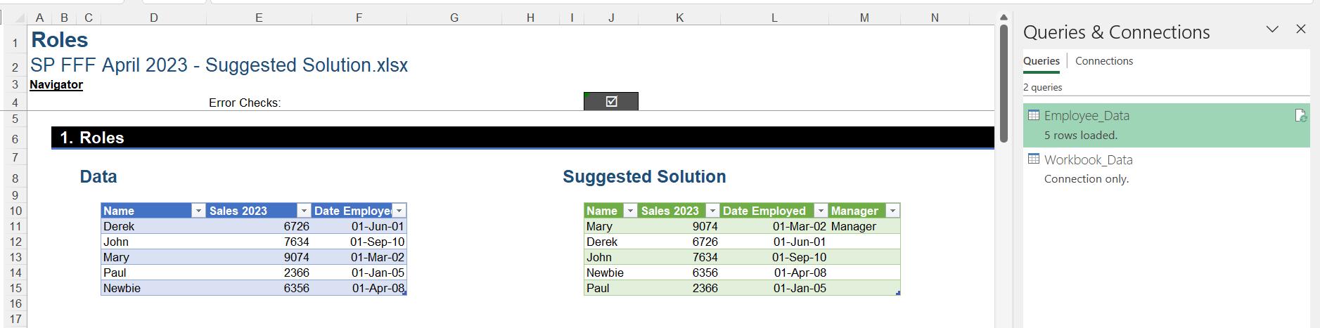
With some minor date formatting, the new Table is complete. 

The Final Friday Fix will return on Friday 26 May 2023 with a new Excel Challenge.  In the meantime, please look out for the Daily Excel Tip on our home page and watch out for a new blog every business working day.