Monday Morning Mulling: December 2021 Challenge

Happy New Year!  On the final Friday of each month, we set an Excel / Power Pivot / Power Query / Power BI problem for you to puzzle over for the weekend.  On the Monday, we publish a solution.  If you think there is an alternative answer, feel free to email us.  We’ll feel free to ignore you.

The special challenge this month was to spill a range of cells that vertically appends two input arrays.  Easy, yes?

The Challenge

Sometimes, you may need to append separate tables into one big table.  To solve this, you may choose to manually copy and paste one table below another or use a more advanced way in Power Query, i.e. Append Queries.

This challenge was designed to make you think outside the box to find another way using only Excel formulas.  You can download the question data here.

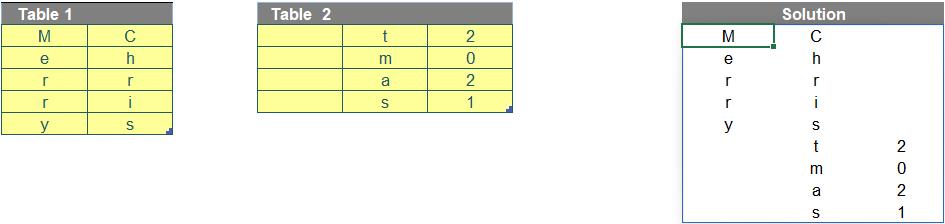
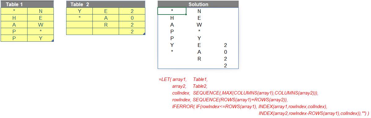
This month’s challenge was to write a formula in one cell using Dynamic Arrays that would spill a range of cells to vertically append two arrays in the file above.  The input tables in the question were different, but the result should look similar to the array generated on the right (below):

As always, there were some requirements:

• the formula needed to be in just one cell (no “helper” cells)
• this was a formula challenge; no Power Query / Get & Transform or VBA!
• the formula needed to be flexible, so that if we adjusted the number of rows and / or columns of the two input tables, the formula should still work
• obviously, the numbers of rows / columns of the output table could not exceed the row / column limitations of Excel.

Suggested Solution

You can find our Excel file here which demonstrates our suggested solution.  However, before explaining our solution, we will clarify how we came up with it first.

Brainstorming

Firstly, we need to consider some features (e.g. numbers of rows and columns) of the output array.  In the question, Table 1 has five [5] rows and two [2] columns, whereas Table 2 has four [4] rows and three [3] columns.

As the two tables are to be combined vertically, the number of rows and columns of the output should be calculated as below:

• Number of rows: 9

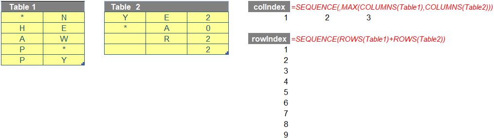
• Number of columns: 3

Secondly, to create a Dynamic Range for the output, we need the help of INDEX and SEQUENCE which you can read more about in this blog.

The row and column index numbers of INDEX need to be created by SEQUENCE as follows.  We will call them rowIndex and colIndex.

Therefore, when we apply the combination of INDEX and SEQUENCE to Table 1, the result will look as below.

Finally, when appending two items, we need to think of something as a connector.  For example, in order to attach two papers together, you may need a piece of tape, a staple or a paper clip.

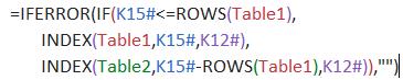
Regarding this challenge, the trick here is to use rowIndex with a simple IF statement (below) as a connector, i.e.

“If rowIndex is less than or equal to the number of rows of Table 1, then get Table 1 else get Table 2.”

The rowIndex numbers of Table2 used in INDEX function need to restart with one [1], so that they are calculated a little bit differently from those of Table1, using the formula below:

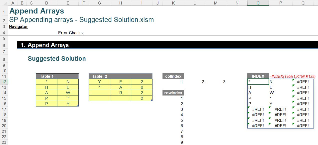
After applying this connector, we will get the result as follows:

You can see that we obtain some #REF! errors, since there is no value of Table 1 in the third column. These are easily fixed by adding an IFERROR function outside the IF statement to replace the resulting errors with blanks (“”).

Returning to the Suggested Solution

You may wonder why the challenge only allows a formula cell when there are a number of working steps above.  Our solution is a combination of all of the described steps above within a LET formula as follows:

There are four variables, namely array1, array2, colIndex and rowIndex:

• array1 and array2 are the two input tables in the question
• colIndex and rowIndex are the index numbers of columns and rows of the output array.

Then, the final part of the formula is the calculation to vertically append two input arrays, viz.

Although it is a long and complex formula, you can apply it to your input tables by only replacing the values of array1 and array2.  Moreover, you can use the similar trick to append arrays horizontally instead of vertically or append more than two arrays.  Feel free to think outside the box and create your own megaformulae.

Happy New Year 2022!

The Final Friday Fix will return on Friday 28 January 2022 with a new Excel Challenge.  In the meantime, please look out for the Daily Excel Tip on our home page and watch out for a new blog every business working day.