
Excel for Mac: Power Query and PivotTables – Consolidate Ranges
16 February 2024
This week in our series about Microsoft Excel for Mac, we show you a better way to create a PivotTable with data from several ranges, sometimes called a Consolidated Range PivotTable.
People using Excel for Mac have requested that Microsoft adds the PivotTable and PivotChart Wizard to Mac so they may create PivotTables that combine, or consolidate, ranges from multiple sheets into a single PivotTable. The wizard exists on Windows, although it’s somewhat hidden. It seems that Microsoft doesn’t want PivotTables to be created this way and that’s fine now that Power Query is available on Mac.
Consolidating Ranges for a PivotTable
Years ago, the way to create a PivotTable based upon multiple ranges from more than one sheet was to use a tool called the ‘PivotTable and PivotChart Wizard’. This article doesn’t go into the details of how to use it, but it allows you to specify ranges from multiple sheets so the data can be combined into a single PivotTable. This wizard isn’t available in Excel for Mac. Even if you’re using Windows, it’s difficult to find (ALT + D + P).
The screen shots below show the wizard on Windows. The last step allows multiple ranges to be combined for use as the data source.
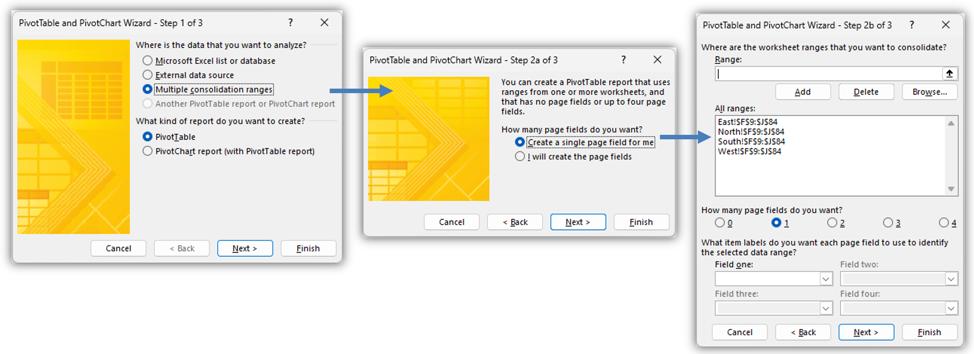
As a tip, in Windows, having pressed ALT + D + P to launch the wizard you can then add it to your QAT (Quick Access Toolbar).
Several new ways
The good news is that even if the wizard were available on Mac, we would still recommend using Power Query or some of the new Excel functions for this scenario.
Power Query is great for combining ranges from multiple sheets, workbook, and other sources. Its flexibility makes it a great choice, and we’ll show an example of how to do this.
Some of the dynamic array functions are also great for combining data. Specifically, you can use VSTACK and HSTACK to append arrays (ranges) together into a single array. Then you can use the new array as the source data for a PivotTable. We’ll show a brief example of this.
Combine ranges with Power Query
Suppose you have sales data on four [4] sheets representing four regions. The steps here can be used to combine them in Power Query so you can use the combined data in a PivotTable. Hopefully, the format of the data on your sheets is consistent, but if it’s not, then Power Query should be able to transform it as needed to make it usable. The same can’t be said for the wizard – your data ranges needed to be in a consistent format.
You can follow along with our example file, provided here.
Just follow these
steps:
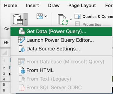
- Create a query for each range: Choose Data -> Get Data (Power Query)
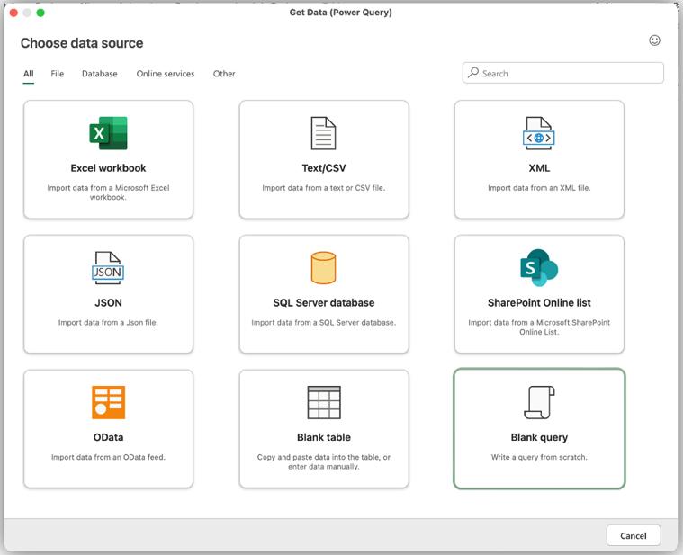
- Choose ‘Blank Query’ from the available data sources
- A new dialog will appear. In the line that says Source = "", replace the double quotes with Excel.CurrentWorkbook() as shown in the screen shot below.
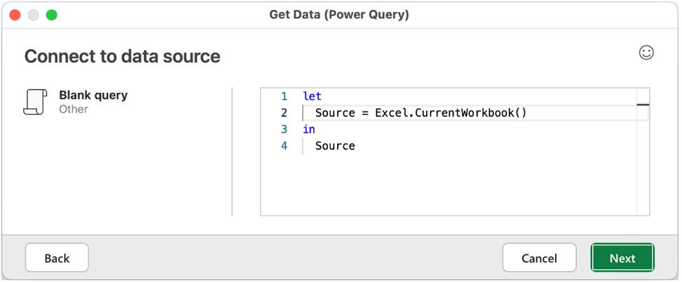
- The code should be exactly as below (it’s case-sensitive):
let
Source = Excel.CurrentWorkbook()
in
Source
- Press Next. The Power Query Editor window will appear. There will be two [2] columns in the table preview, Content and Name. The Content column will have [Table], which means that each row contains a table or range of data. The Name column shows the name of each table or range
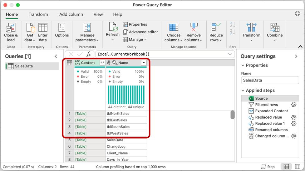
- Rename your query to a meaningful name rather than the default name provided. Do this by typing in the Name field in the Query settings pane on the right side. This step is optional and won’t affect your data, but the name will be visible when you create your PivotTable.
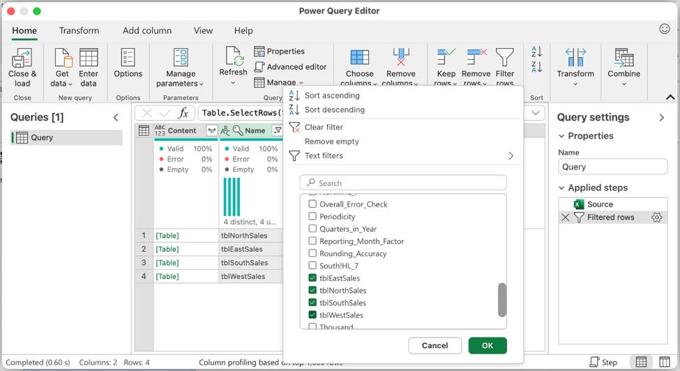
- Click the Filter button in the header of the Name column. In our example, we have tables called tblEastSales, tblNorthSales, tblSouthSales and tblWestSales. We only want those tables to be included in our data set, so we de-select all the other tables. The fastest way is to click the ‘Select all’ item, which removes all the tick marks. Then tick the tables that you want. Press OK
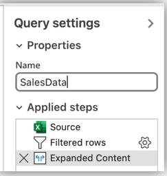
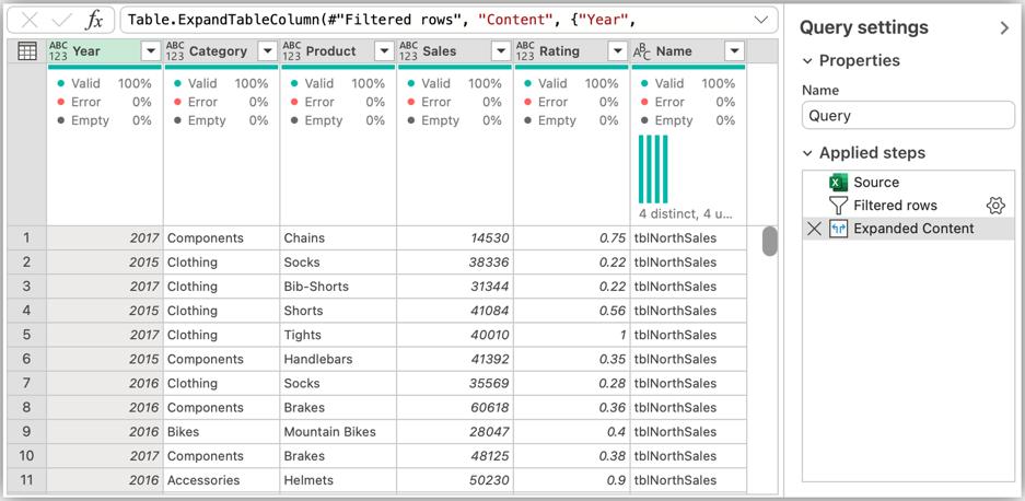
- Expand the Content column. Do this by pressing the button on the right side of the column header, then press OK.
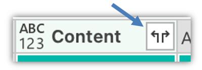
- The screen shot below shows the Expand button being clicked in the header of the Content column. The dialog shows the available columns that will be included in the expanded data. If any of the columns aren’t needed for your PivotTable, you can de-select them. Notice that the Name column shows the table name that was the source range for each value
- If needed, you can use all the other features of Power Query to transform your data. You can’t do any of that with the wizard, which is why Power Query is a great alternative
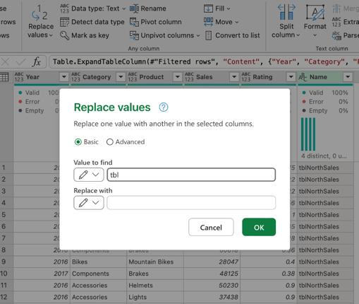
- In our example, we want to simplify the values in the Name column (region). Since the table names are like tblNorthSales, we want to get rid of “tbl” and “sales”. Press the ‘Replace Values’ button, then type “tbl” in the ‘Value to find’ field and leave the ‘Replace with’ field empty. Remove the word “Sales” in a similar way to be left with just the region. Power Query applies these steps to all the data, so we only need to do it once
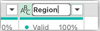
- You may want to rename a column if it makes sense. In our example, we want to rename the Name column to Region, since that’s what we’ll see in our PivotTable. Just double-click on the column header and type the new name
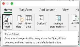
- After you’ve added any other steps you want, press the ‘Close & load’ button on the Ribbon
- Your data will be loaded to a new worksheet or the ‘Load Data’ dialog may appear (as of this writing, the dialog is not available on Mac)
- Now you can create your PivotTable with the combined data from all the ranges.The Region column allows us to use the Region in our PivotTable, even though it’s not in the source tables that we combined
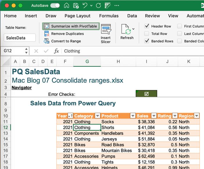
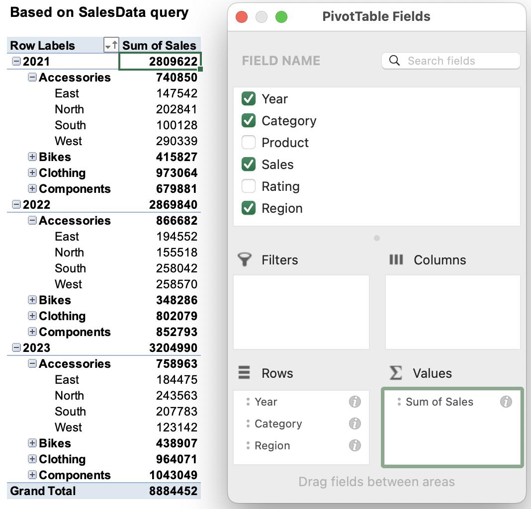
Here, you can see our PivotTable after combining our ranges and adjusting the region field to be more readable.
Combine Ranges with Array formulae
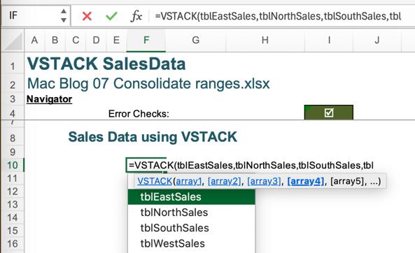
Another way to combine your ranges is by using the VSTACK function. In our example, it’s very simple to combine the ranges by using the following formula:
=VSTACK(tblEastSales,tblNorthSales,tblSouthSales,tblWestSales)
Since our sales tables have names like tblEastSales, it’s easy to just list the tables that we want, and they all get combined into a large data set.
If you use this method, you’ll likely want to add some data, such as column headers, and a column to each table to show the region.
There are a few ways you can add the region, such as:
=HSTACK(VSTACK(tblEastSales,tblNorthSales,tblSouthSales,tblWestSales),
VSTACK(
MAKEARRAY(ROWS(tblEastSales),1,LAMBDA(r,c,"East")),
MAKEARRAY(ROWS(tblNorthSales),1,LAMBDA(r,c,"North")),
MAKEARRAY(ROWS(tblSouthSales),1,LAMBDA(r,c,"South")),
MAKEARRAY(ROWS(tblWestSales),1,LAMBDA(r,c,"West"))))
To add the column headers, you could either just type the headers in the row above the formula, or you can add to the formula, such as:
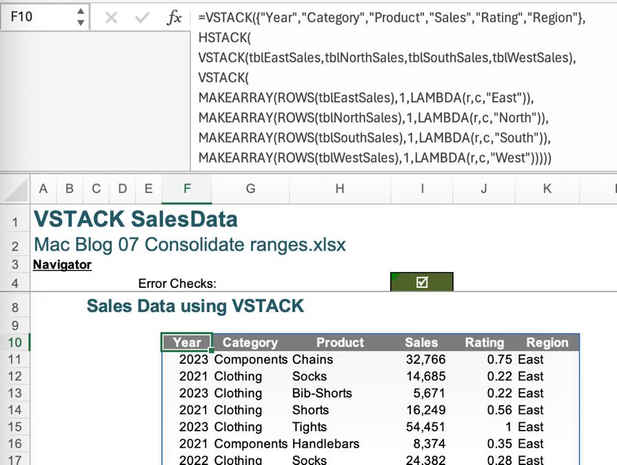
=VSTACK({"Year","Category","Product","Sales","Rating","Region"},
HSTACK(VSTACK(tblEastSales,tblNorthSales,tblSouthSales,tblWestSales),
VSTACK(
MAKEARRAY(ROWS(tblEastSales),1,LAMBDA(r,c,"East")),
MAKEARRAY(ROWS(tblNorthSales),1,LAMBDA(r,c,"North")),
MAKEARRAY(ROWS(tblSouthSales),1,LAMBDA(r,c,"South")),
MAKEARRAY(ROWS(tblWestSales),1,LAMBDA(r,c,"West")))))
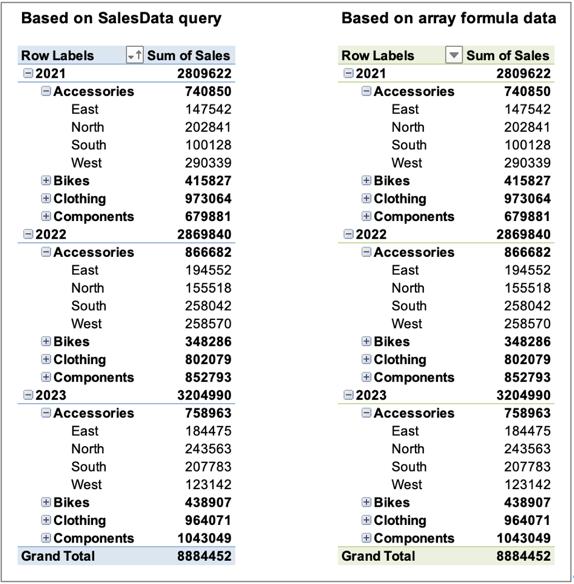
Here, our screen shot shows two [2] PivotTables that have the same values. The data source for one is the SalesData query that we created in Power Query, and the data source for the other is the array formula described above.
We hope you find this topic helpful. Check back for more details about Excel for Mac and how it’s different to Excel for Windows.