14 New Excel Functions

Microsoft doesn’t want to do things by halves, does it?  Yesterday saw the announcement of no less than 14 (!)new Excel functions designed to help manipulate text and arrays in your worksheets.  If only we could find some that would massage the financial as well…

Now, before I go any further, let me be completely clear about availability.  At the time of writing, these functions are currently only available to users running Beta Channel, Version 2203 (Build 15104.20004) or later on Windows and Version 16.60 (Build 22030400) or later on Mac.  Even then, the availability is “flighted”.  Here at SumProduct HQ, we have had to get clever with virtual machines to get our grubby little hands on them, so please don’t despair if you can’t access them yet.  They are definitely circulating!!

In summary, the functions are essentially grouped as follows:

• text manipulation
• combining arrays
• shaping arrays
• resizing arrays.

Let’s take a look at each of these four subsets in turn.

Text Manipulation Functions

We have talked about the common text manipulation functions such as FIND, LEFT, LEN, MID, RIGHT, SEARCH and SUBSTITUTE before but these new functions allow you to dismember text strings without requiring a PhD in Astrophysics.

If it TEXT you too long to understand these older functions, then you needn’t worry anymore.  There are three new functions that may help here:

1. TEXTBEFORE: returns text that’s before delimiting characters
2. TEXTAFTER: returns text that’s after delimiting characters
3. TEXTSPLIT: splits text into rows or columns using delimiters.

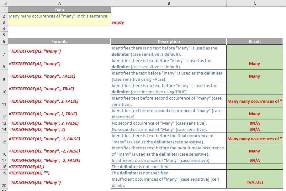
The TEXTBEFORE function

The TEXTBEFORE function returns the string of text that occurs before a given substring (i.e. a character or set of characters) in that string.  It is the opposite of the TEXTAFTER function.  TEXTBEFORE has the following syntax:  

The TEXTBEFORE function has the following arguments:

• text: this is required and represents the text string you are searching within.  Wildcard characters are not allowed
• delimiter: this is also required and represents the text in the text string that marks the point before which you wish to extract
• instance number: this is the first optional argument and denotes the nth instance of the delimiter before which you wish to extract.  By default, this is equal to one [1].  If a negative number is used here, the function starts searching for the delimiter from the end rather than the beginning
• ignore case: this too is an optional argument and determines whether the search is case sensitive or not.  The default is TRUE, which means the search for the delimiter is case insensitive; explicitly use FALSE to make the search case sensitive.

It should be further noted that:

• Excel should return an #N/A error if the delimiter is an empty string, but the current Beta version appears to return a blank
• Excel returns an #VALUE! error if the instance number is zero (the default is one)
• Excel returns an #N/A error if the delimiter does not occur within the text
• Excel returns an #N/A error if the instance number is greater than the number of occurrences of the delimiter within the text.

Please see the examples below:

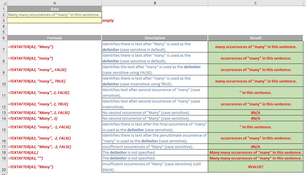
The TEXTAFTER function

The TEXTAFTER function returns the string of text that occurs after a given substring (i.e. a character or set of characters) in that string.  It is the opposite of the TEXTBEFORE function.  TEXTAFTER has the following syntax:  

The TEXTAFTER function has the following arguments:

• text: this is required and represents the text string you are searching within.  Wildcard characters are not allowed
• delimiter: this is also required and represents the text in the text string that marks the point after which you wish to extract
• instance number: this is the first optional argument and denotes the nth instance of the delimiter after which you wish to extract.  By default, this is equal to one [1].  If a negative number is used here, the function starts searching for the delimiter from the end rather than the beginning
• ignore case: this too is an optional argument and determines whether the search is case sensitive or not.  The default is TRUE, which means the search for the delimiter is case insensitive; explicitly use FALSE to make the search case sensitive.

• It should be further noted that:
• Excel should return an #N/A error if the delimiter is an empty string, but the current Beta version appears to return a blank
• Excel returns an #VALUE! error if the instance number is zero (the default is one)
• Excel returns an #N/A error if the delimiter does not occur within the text
• Excel returns an #N/A error if the instance number is greater than the number of occurrences of the delimiter within the text.

Please see relevant examples below:

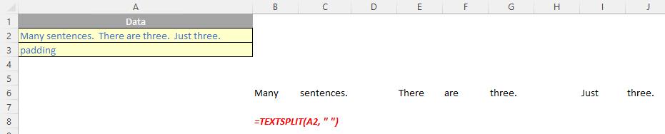
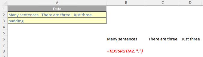
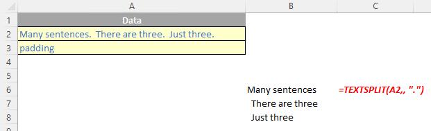
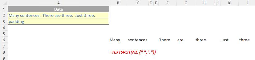
The TEXTSPLIT function

The TEXTSPLIT function is intended to work like the Text to Columns button on the Data tab of the Ribbon, almost like the “inverse” of the TEXTJOIN function.  It allows you to split a given text across rows or down columns.  TEXTSPLIT has the following syntax:  

The TEXTSPLIT function has the following arguments:

• text: this is required and represents the text string you wish to split
• column delimiter: this is optional and denotes one or more characters that specify where to spill the text across columns
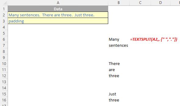
• row delimiter: this is optional and denotes one or more characters that specify where to spill the text down rows
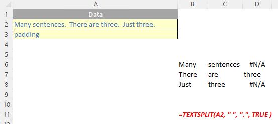
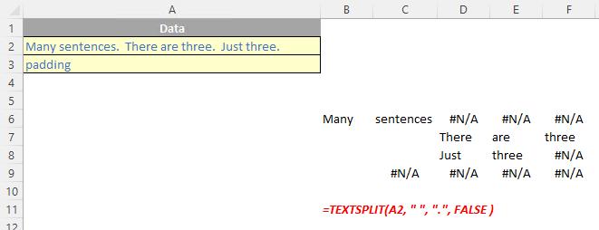
• ignore empty: another optional argument, you should specify TRUE to create an empty cell when two delimiters are used.  This argument defaults to FALSE, which means don't create an empty cell
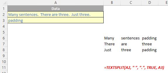
• pad with: not to be confused with Pad Thai, this final optional argument “pads” the resulting text range where cells would otherwise be blank.  The default is N/A.

If there is more than one delimiter (row or column), then an array constant must be used.  For example, to split by both a comma (,) and a period (full stop, .), use =TEXTSPLIT(text, {",", "."}).

Just for a change, some more examples:

Combining Arrays

Since end users have been playing with arrays more and more, it has become noticeable that it can be quite challenging to combine data, especially when their sources are flexible in size.  There are two new functions that may assist:

1. HSTACK: combine dynamic arrays, stacking horizontally
2. VSTACK: combine dynamic arrays, stacking vertically.

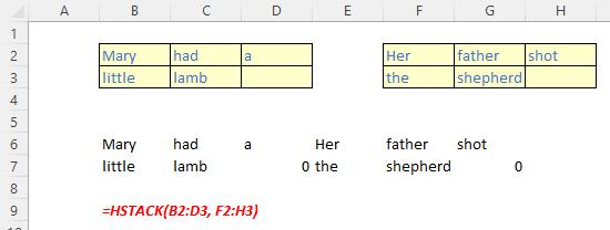
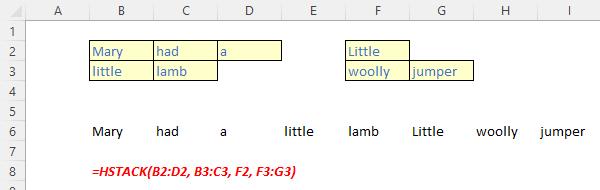
The HSTACK function

The HSTACK function returns the array formed by appending each of the array arguments in a column-wise fashion (Microsoft’s jargon, not ours).  It has the following syntax:  

The HSTACK function has the following argument(s):

• array: the first argument is required (others are optional) and represents the array(s) to append.
• It should be noted that:
• HSTACK returns the array formed by appending each of the array arguments in a column-wise fashion.  The resulting arraywill be the following dimensions:
  • columns: the maximum of the column count from each of the array arguments
  • rows: the combined count of all the rows from each of the array arguments

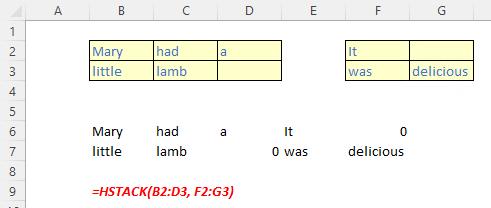
Excel returns an #N/A error if an array has fewer rows or columns than the maximum in any selected array.  To remove the errors, you should use the IFERROR function.

Please see my the following examples:

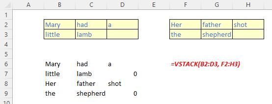
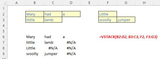
The VSTACK function

The VSTACK function returns the array formed by appending each of the array arguments in a row-wise fashion (Microsoft’s jargon, not ours).  It has the following syntax:  

The VSTACK function has the following argument(s):

• array: the first argument is required (others are optional) and represents the array(s) to append.

It should be noted that:

• VSTACK returns the array formed by appending each of the array arguments in a row-wise fashion.  The resulting arraywill be the following dimensions:
  • rows: the maximum of the row count from each of the array arguments
  • columns: the combined count of all the columns from each of the array arguments
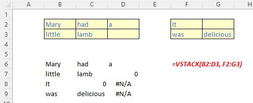
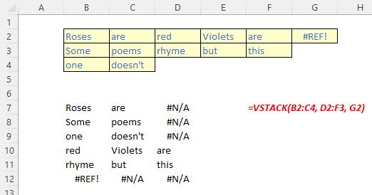
• Excel returns an #N/A error if an array has fewer rows or columns than the maximum in any selected array.  To remove the errors, you should use the IFERROR function.

Some illustrations:

Shaping Arrays

Changing the “shape” of data in Excel, especially from arrays to lists and vice versa, is a popular request with our clients and is difficult to achieve formulaically (Power Query makes it nice and easy though!).  This is where the next four functions come into play:

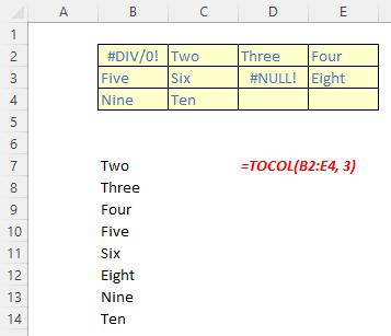
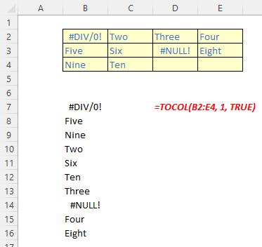
1. TOCOL: convert a two-dimensional array into a single column (list) of data
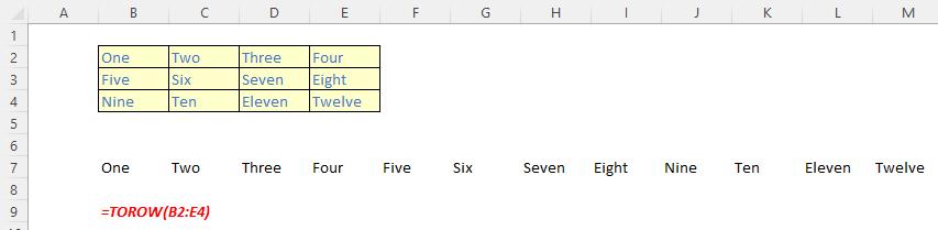
2. TOROW: convert a two-dimensional array into a single row (list) of data
3. WRAPCOLS: creates a two-dimensional array of a specified height by wrapping data from a column (list) of data once the prescribed height is achieved (this is essentially the opposite of the TOCOL or TOROW functions)
4. WRAPROWS: creates a two-dimensional array of a specified width by wrapping data from a row (list) of data once the prescribed width is achieved (this is essentially the opposite of the TOCOL or TOROW functions).

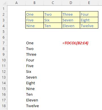
The TOCOL function

The TOCOL function returns a column vector containing all of the items in the source array.  It has the following syntax:  

The TOCOL function has the following arguments:

• array: this is required and denotes the array or reference to return as a column
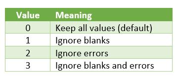
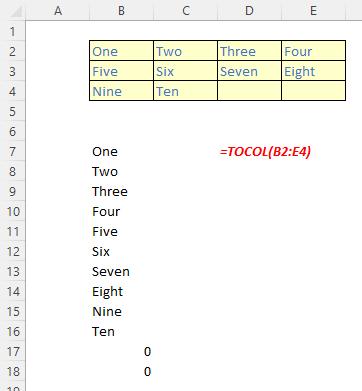
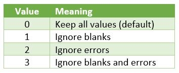
• ignore: this is optional and identifies whether to ignore certain types of values; by default, no values are ignored.  The omissions are governed as follows:

• scan by column: this is optional and sets the scan of the array by column.  However, by default, the array is scanned by row.

It should be noted that:

• if scan by column is omitted or FALSE, the array is scanned by row; if TRUE, the array is scanned by column
• Excel returns an #VALUE! error when an array constant contains one or more numbers that are not a whole number
• Excel returns an #NUM! error when array becomes too large.

Just for a change, some examples:

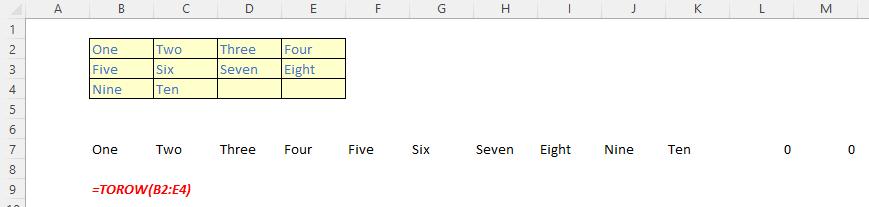
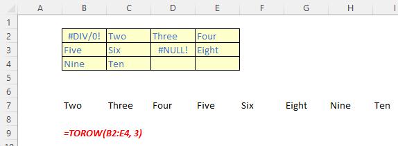
The TOROW function

The TOROW function returns a row vector containing all of the items in the source array.  It has the following syntax:  

The TOROW function has the following arguments:

• array: this is required and denotes the array or reference to return as a row
• ignore: this is optional and identifies whether to ignore certain types of values; by default, no values are ignored.  The omissions are governed as follows:

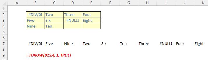
• scan by column: this is optional and sets the scan of the array by column.  However, by default, the array is scanned by row.

It should be noted that:

• if scan by column is omitted or FALSE, the array is scanned by row; if TRUE, the array is scanned by column
• Excel returns an #VALUE! error when an array constant contains one or more numbers that are not a whole number
• Excel returns an #NUM! error when array becomes too large.

Some illustrations:

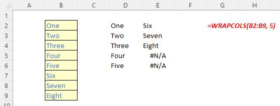
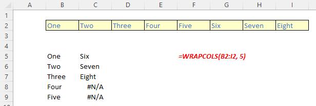
The WRAPCOLS function

The WRAPCOLS function wraps the provided vector by columns after a specified number of elements.  It has the following syntax:  

The WRAPCOLS function has the following arguments:

• vector: this is required and denotes the row or column vector / reference to wrap
• wrap count: this is also required and represents the maximum number of values (depth / height) for each column
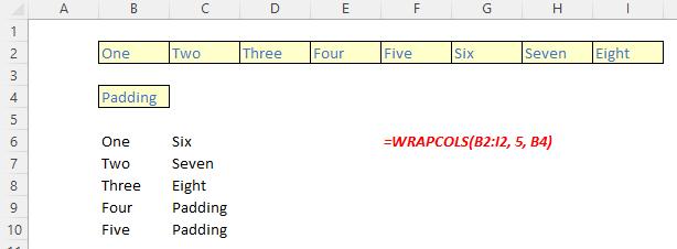
• pad with: this is optional and defines the value with which to pad.  The default is N/A.

It should be noted that:

• the elements of the vector are placed into a two-dimensional array by column
• each column has wrap count elements
• the column is padded with pad width if there are insufficient elements to fill it
• if wrap count is greater or equal to the number of elements in vector, then the vector is simply returned as the column vector result of the function
• Excel returns an #VALUE! error when vector is not a one-dimensional array
• Excel returns an #VALUE! error when wrap count is less than one [1] or is not an integer.

Please see the following examples:

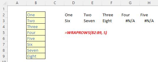
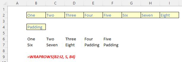
The WRAPROWS function

The WRAPROWS function wraps the provided vector by rows after a specified number of elements.  It has the following syntax:  

The WRAPROWS function has the following arguments:

• vector: this is required and denotes the row or column vector / reference to wrap
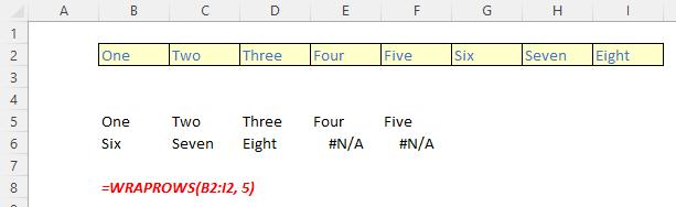
• wrap count: this is also required and represents the maximum number of values (width) for each row
• pad with: this is optional and defines the value with which to pad.  The default is N/A.

It should be noted that:

• the elements of the vector are placed into a two-dimensional array by row
• each row has wrap count elements
• the row is padded with pad width if there are insufficient elements to fill it
• if wrap count is greater or equal to the number of elements in vector, then the vector is simply returned as the row vector result of the function
• Excel returns an #VALUE! error when vector is not a one-dimensional array
• Excel returns an #VALUE! error when wrap count is less than one [1] or is not an integer.

More examples:

Resizing Arrays

The final array manipulation covered by this myriad of new functions concerns resizing.  This is where the last five functions prove useful:

1. CHOOSECOLS: returns the specified rows from an array
2. CHOOSEROWS: returns the specified columns from an array
3. DROP: drops rows or columns from an array start or end
4. EXPAND: expands an array to the specified dimensions
5. TAKE: returns rows or columns from the start or end of an array.

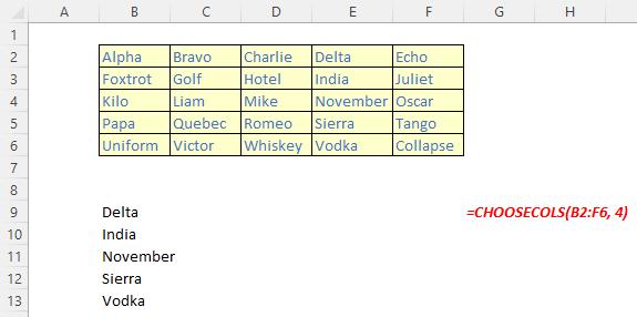
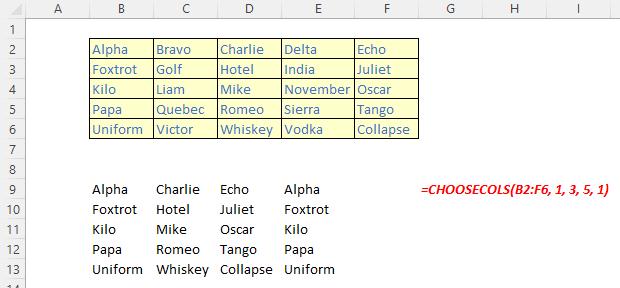
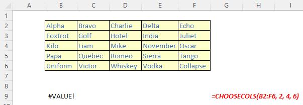
The CHOOSECOLS function

The CHOOSECOLS function returns the specified columns from an array.  It has the following syntax:  

The CHOOSECOLS function has the following arguments:

• array: this is required and represents the selected array
• column number 1: this is also required and denotes the column number of the first column to be returned
• column number 2: this and subsequent arguments are optional.  This / these represent(s) the second and subsequent column numbers to be returned.

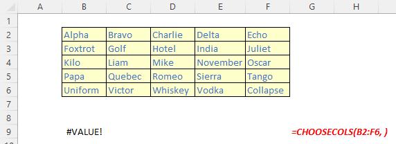
It should be noted that Excel will return an #VALUE! error if the absolute value of any of the column number arguments is zero or exceeds the number of columns in the array.

Some examples:

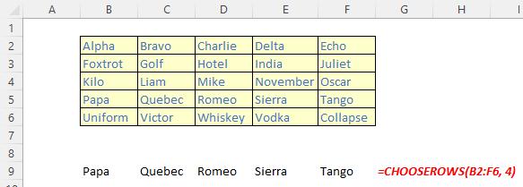
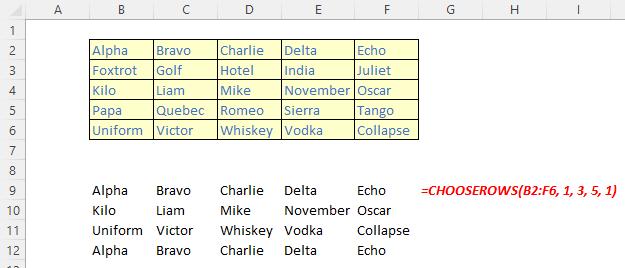
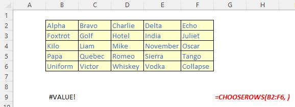
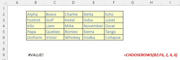
The CHOOSEROWS function

The CHOOSEROWS function returns the specified rows from an array.  It has the following syntax:  

The CHOOSEROWS function has the following arguments:

• array: this is required and represents the selected array
• row number 1: this is also required and denotes the row number of the first row to be returned
• row number 2: this and subsequent arguments are optional.  This / these represent(s) the second and subsequent row numbers to be returned.

It should be noted that Excel will return an #VALUE! error if the absolute value of any of the row number arguments is zero or exceeds the number of rows in the array.

Illustrations:

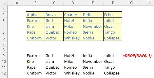
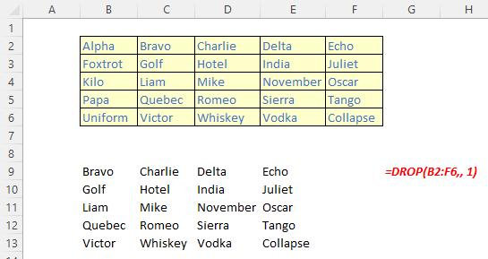
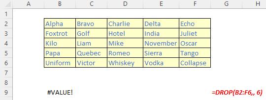
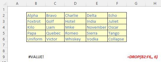
The DROP function

The DROP function excludes a specified number of contiguous rows or columns from either the start or the end of an array.  It has the following syntax:  

The DROP function has the following arguments:

• array: this is required and represents the selected array from which to drop the rows or columns
• rows: this is also required and denotes the number of rows to drop (exclude) from the top.   If this number is negative, the values drop from the bottom of the array
• columns: this is optional and denotes the number of columns to drop (exclude).   If this number is negative, the values drop from the end of the array.

It should be noted that:

• when rows or columns are not provided or missing, all rows and columns are returned
• if the absolute value of rows or columns is greater than the number of rows or columns in the array, then all rows or columns are supposed to be returned, but presently #VALUE! appears to be the favoured treatment
• Excel returns an #CALC! error to indicate an empty array when rows or columns is zero [0]
• Excel returns an #NUM! when array is too large.

Please see the examples below:

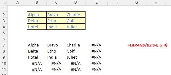
The EXPAND function

The EXPAND function expands (or pads) an array to specified row and column dimensions.  It has the following syntax:  

The EXPAND function has the following arguments:

• array: this is required and represents the selected array to be expanded
• rows: this is also required and denotes the number of rows in the expanded array.  If this argument is missing (not bad for a required argument!), rows will not be expanded
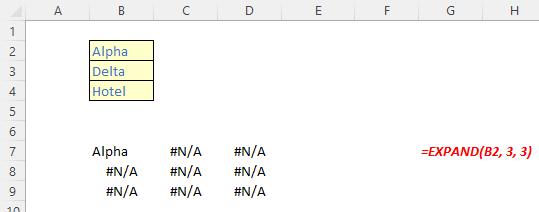
• columns: this is optional and denotes the number of columns in the expanded array.  Again, should columns not be specified, this dimension will not be expanded
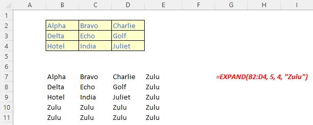
• pad with: this is an optional value with which to pad.  The default is N/A.

It should be noted that:

• if rows isn’t provided or is empty, the default value is the number of rows in the array argument (as aforementioned)
• if columns isn’t provided or is empty, the default value is the number of columns in the array argument
• if pad with is not provided and array has one value for that dimension, then that value is used.  This operation is commonly referred to as array “broadcasting”; however, this does not appear to work presently
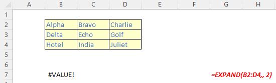
• Excel returns an #VALUE! error when the rows or columns argument is less than the rows or columns in the array argument
• Excel returns an #N/A error when pad with is greater than a single column or row
• Excel returns an #NUM! when array is too large.

Please see our penultimate examples below:

The TAKE function

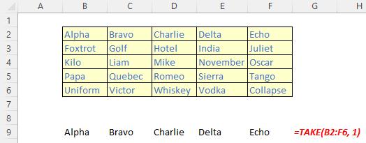
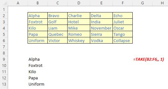
The TAKE function returns a specified number of contiguous rows or columns from either the start or the end of an array.  It has the following syntax:  

The TAKE function has the following arguments:

• array: this is required and represents the selected array from which to take (extract) the rows or columns
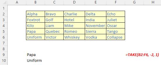
• rows: this is also required and denotes the number of rows to take from the top.   If this number is negative, the values are taken from the bottom of the array
• columns: this is optional and denotes the number of columns to take.   If this number is negative, the values take from the end of the array also.

It should be noted that:

• when rows or columns are not provided or missing, all rows and columns are returned
• if the absolute value of rows or columns is greater than the number of rows or columns in the array, then all rows or columns are supposed to be returned, but presently #VALUE! appears to be the favoured treatment
• Excel returns an #CALC! error to indicate an empty array when rows or columns is zero [0]
• Excel returns an #NUM! when array is too large.

Please see the final examples below:

Word to the Wise

These functions are “hot off the press” and presently “in Beta”, so it is possible they may change and / or their behaviour may be modified.  This should not deter you from trying these out.  Compared to the recent onslaught of LET and LAMBDA related functions, the concepts in play are reasonably simple to understand and could prove highly useful for those looking to work with arrays more in Excel.

Bring on the next batch!