Charts and Dashboards: Tornado Charts - Part 3

Welcome back to our Charts and Dashboards blog series.  This week, we’ll finalise the formatting of our Tornado chart.

Last week, we finished preparing our data, ready to graph.  However, when put into a bar chart it didn’t look quite finished yet.

This week we’ll cover step by step the process of taking last week’s data and achieving the signature Tornado chart look.  

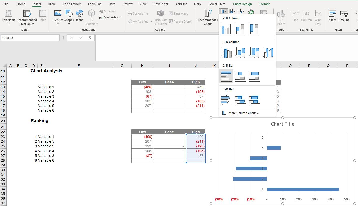
First, we want to highlight the ranked High data and create a bar graph.

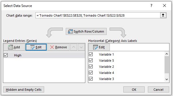
It’s important to ensure that accurate axis labels are used.  Therefore, we right click on the graph and choose ‘Select Data’ so that we can edit the ‘Horizontal (Category) Axis Labels’ to select the variable names.  

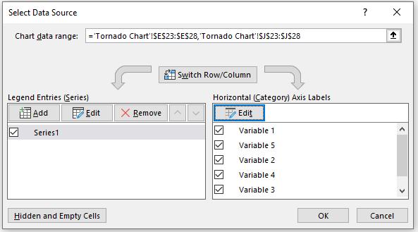
We also want to edit the ‘Legend Entries (Series)’ to ensure that ‘Series 1’ has a more sensible name.  Here, I’ll choose the column header of ‘High’.

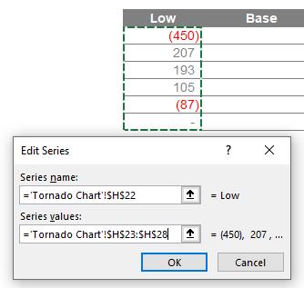
We now want to add a series for the ‘Low’ data, again ensuring it is appropriately named.

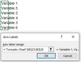
We also will want to adjust the Horizontal Axis Labels again.

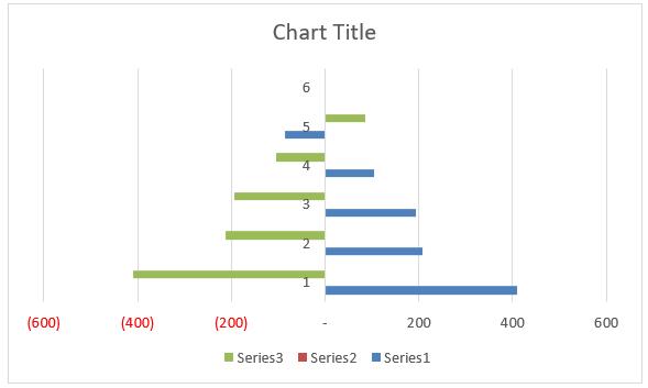
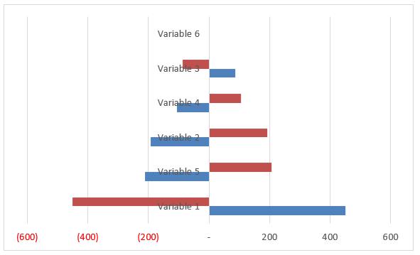
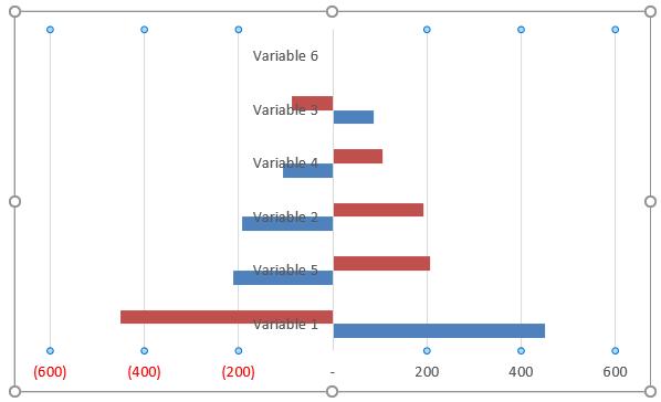
This will give us something that looks vaguely like a Tornado chart, but there is definitely some work to do.

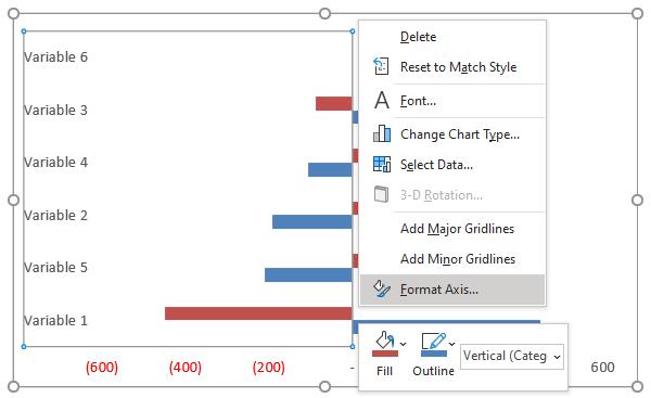
We can begin by removing the ‘Horizontal (Value) Axis Major Gridlines’, this can be done simply by clicking on them in the graph area and pressing delete.

Next we want to format the y-axis, so we right click on the axis and choose ‘Format Axis’.

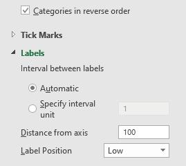
We want the labels to be in the ‘Low’ position with the categories in reverse order, which you will locate on ‘Axis Options’ in ‘Axis Options’ (!).

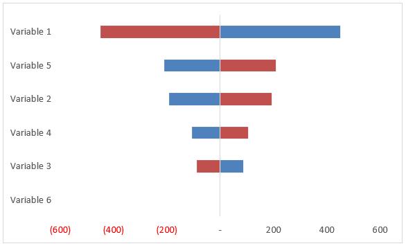
The graph is now starting to come together!  However, we don’t want the number labels at the top.

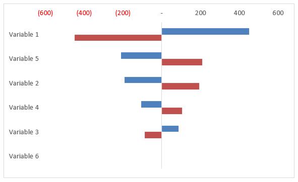
We can right-click on this axis, choose ‘Format Axis’, and change the label position to High.  This might seem unusual, but as we reversed the order of the labels earlier, ‘High’ will now put this label at the bottom.

Next we’ll want to select the data and adjust the series overlap.

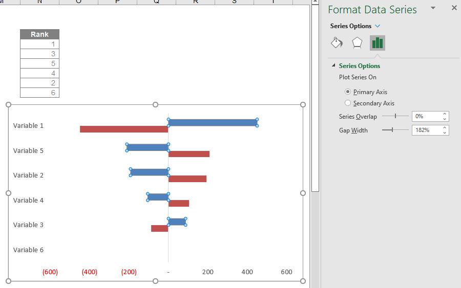
We can set this to 100%, making the bars in line with one another.

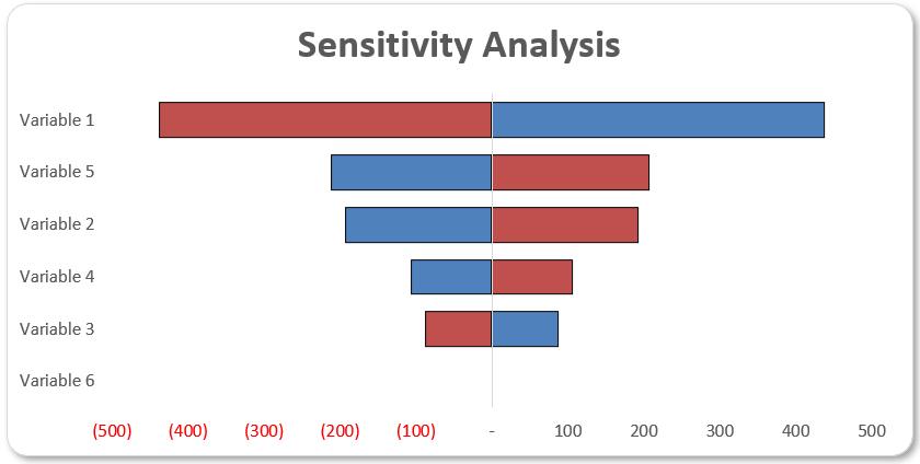
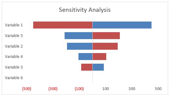
And there you have it, a Tornado chart! Other formatting can be considered, such as adding a title, adjusting the series width or any of the various options available in Excel.  

One thing to note…  In later versions of Excel, take a detailed look at ‘Recommended Charts’.  You may even find what you are looking for without making any of these changes.  Excel is moving on!

That’s it for this week.  Come back next week for more Charts and Dashboards tips.