
Charts and Dashboards: Rolling Charts
4 December 2020
Welcome back to this week’s Charts and Dashboards blog series. This week, we consider rolling charts, whatever they may be...
A “rolling” chart is just like a rolling budget: it displays the last x months (typically, the past 12 months), but keeps up to date automatically. The idea is similar, but not quite the same, as we do not wish to extend the range, simply keep moving the 12 months along the time axis.
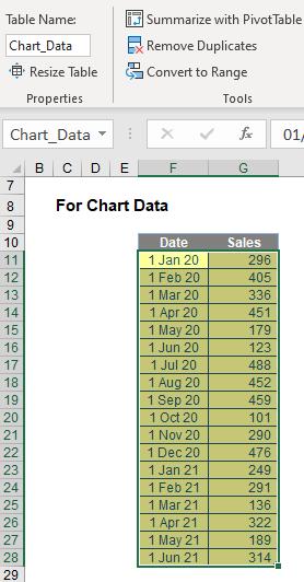
To do this, you still create a Table (mine is labelled ‘Chart_Data’):
I then calculate the latest date in the formula by typing =MAX( and then highlighting cells F11:F28 in my example. This gives me the formula
=MAX(Chart_Data[Date])
The great thing about this formula expressed in this way is as the dates extend, the range will update automatically. I use this formula in the final row of a second table (check out cell L22 in the image below):
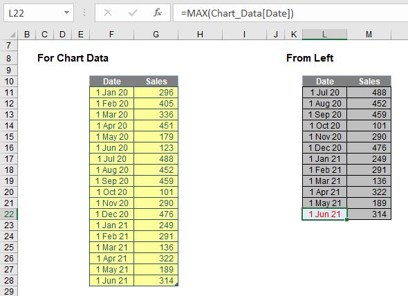
To populate the rest of the data in column L, in cell L21 I write the following formula
=EDATE(L22,-1)
This generates the same day of the month one month earlier. I then copy this formula into cells L11:L20. Finally, I use a LOOKUP formula to derive the Sales data. For example, the formula in the final period here is
=LOOKUP(L22,Chart_Data)
Here, the LOOKUP formula will always look for the date in the first column of Chart_Data and return the value in the final (second) column. You should note that this chart data table is always 12 rows deep for a 12-month look-back. If you need a rolling budget for a different duration, simply amend the number of rows accordingly. It is this table that populates the chart:
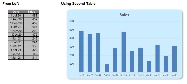
It's pretty straightforward and this example is included in the attached example file.
That’s it for this week. Check back next week for more Charts and Dashboards tips.