
Charts and Dashboards: Bullet Charts – Part 3
5 March 2021
Welcome back to this week’s Charts and Dashboards blog series. This week, we complete our take on Bullet Charts.
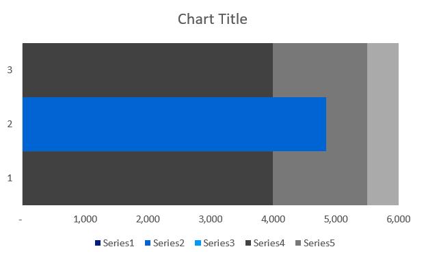
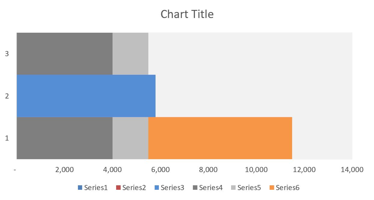
In the past few weeks, we have analysed and created the initial bullet chart, and then formatted it to get a chart similar to the one below:
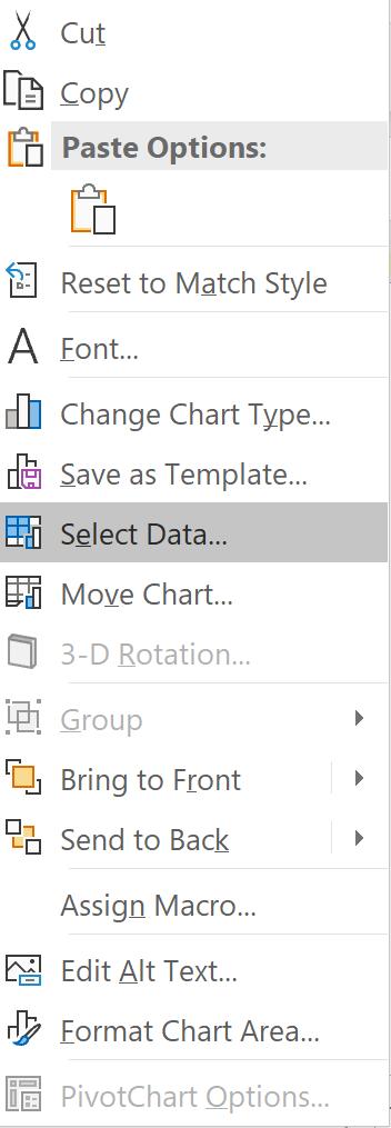
Now, to insert the Target bar, right click on the chart select ‘Select Data’ menu:
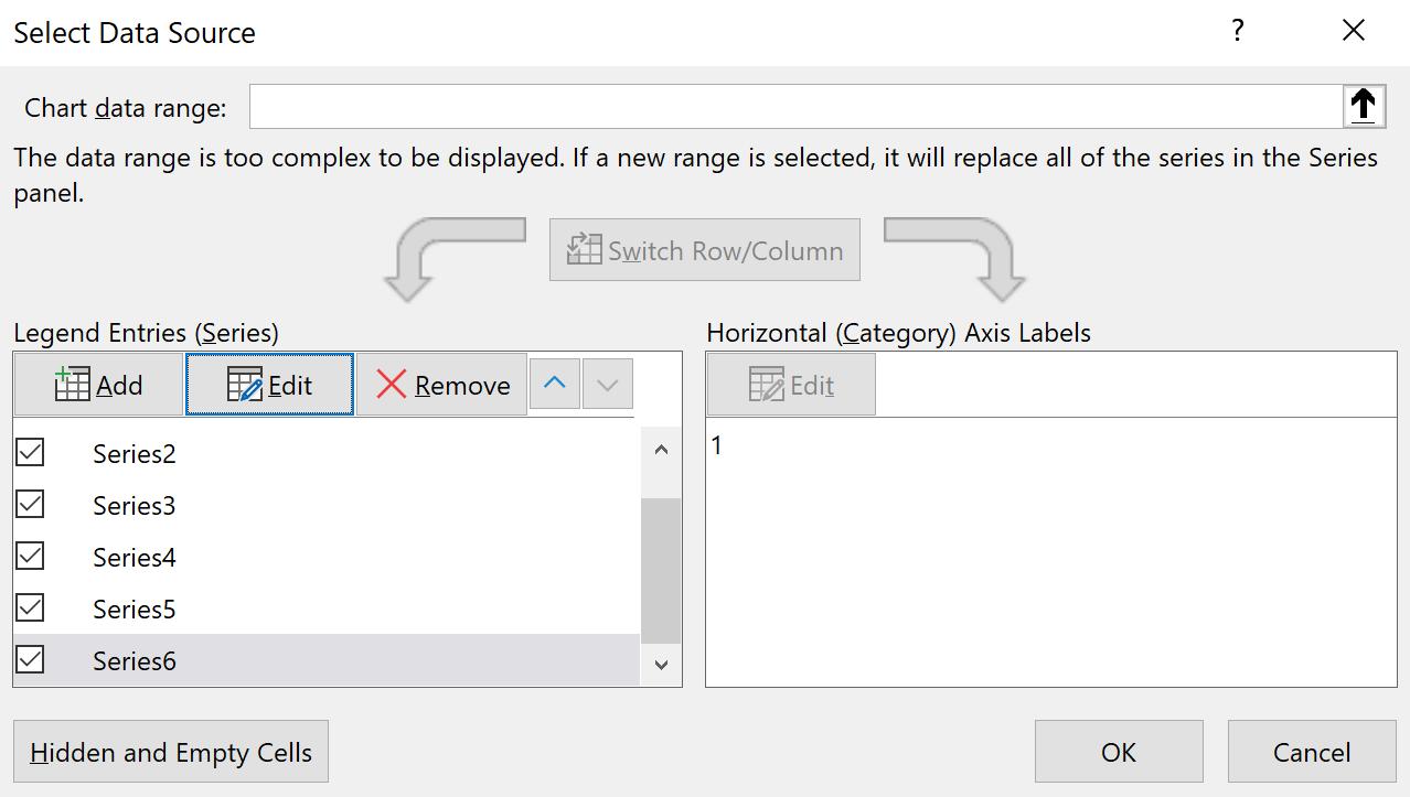
This will bring up the ‘Select Data Source’ dialog box:
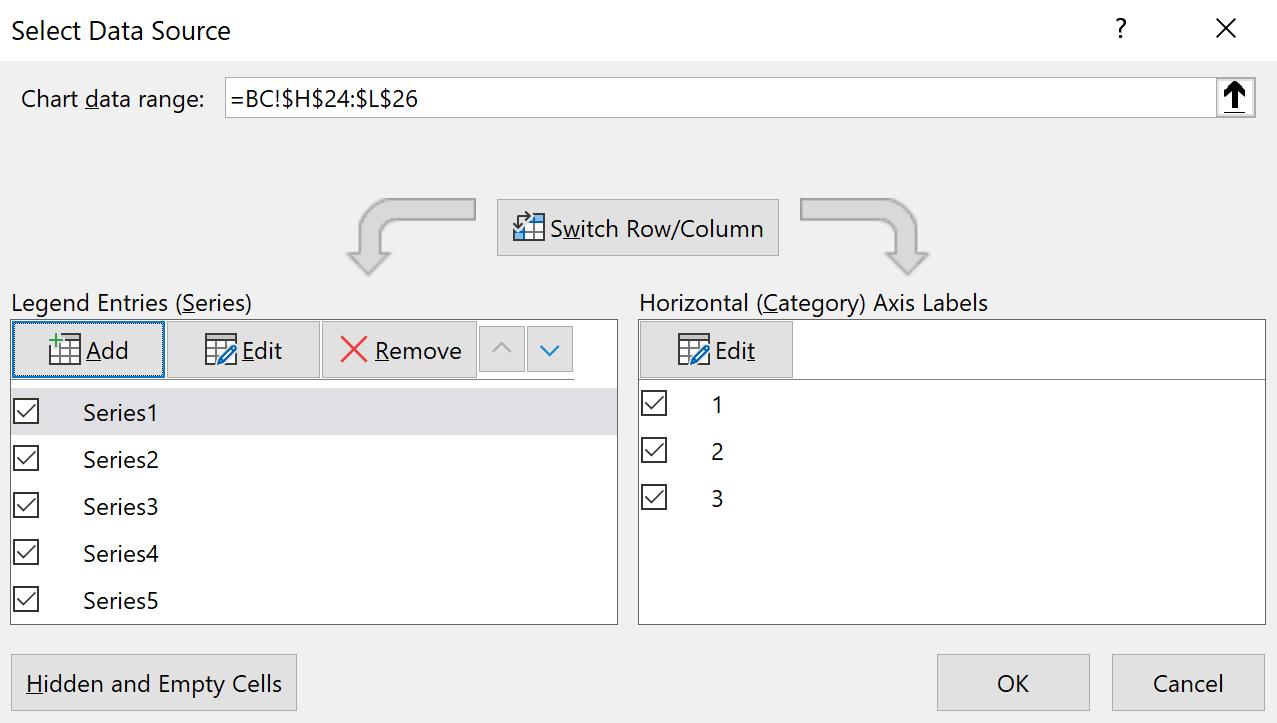
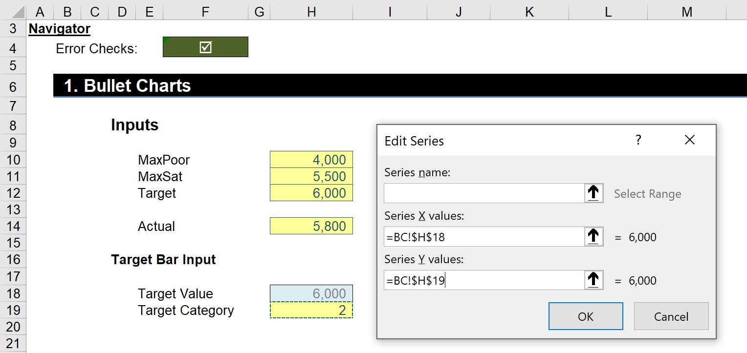
Click on the Add option. This will bring up the ‘Edit Series’ dialog box:
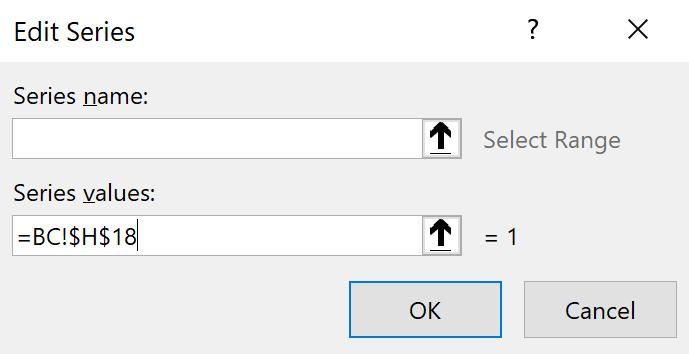
Input =BC!$H$18 into the series values area, then click OK. The chart may look like something like this now:
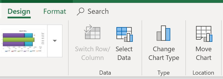
Highlight any series in the chart then navigate to the Design tab on the Ribbon and select ‘Change Chart Type’.
This will bring up the ‘Change Chart Type’ dialog box:
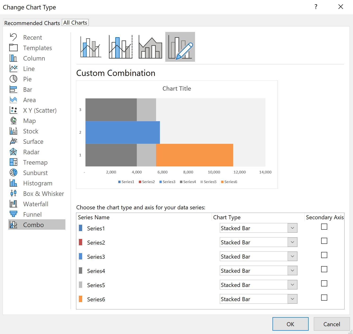
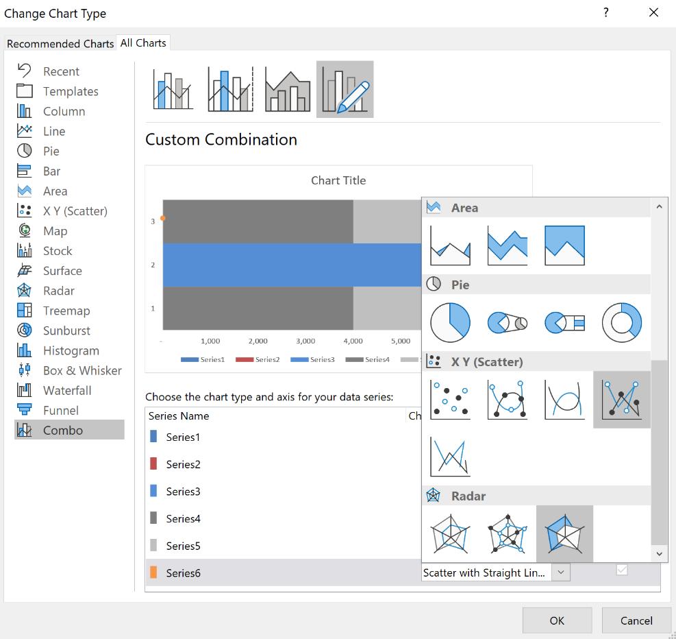
Make sure that you are on the Combo chart option, look for Series6 (this should be the new series that we just added). Change the chart type to ‘Scatter with Straight Line’:
Now, right click on the chart and select ‘Select Data’, navigate to Series6 in the ‘Legend Entries (Series)’ and click Edit:
This will bring up the ‘Edit Series’ dialog box. We can now plot the ‘Target Category’ as the ‘Series Y values’ and the ‘Target Value’ as the ‘Series X values’:
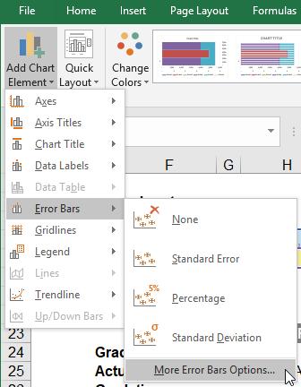
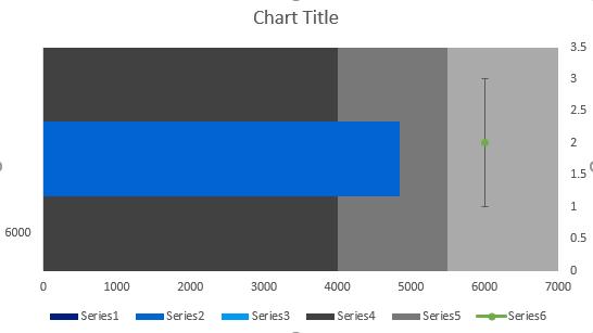
Select Series6 with the side panel, navigate to the ‘Design’ tab on the Ribbon and select the ‘More Error Bar Options’ from the ‘Add Chart Element’ option.
The error bar will look like this:
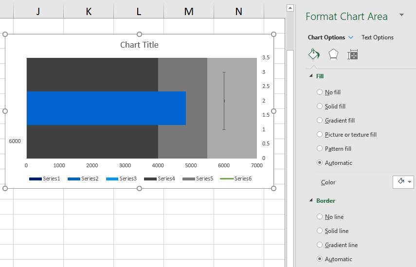
We will have to get rid of the marker. Navigate to the ‘Format Chart Area’ side panel and toggle ‘No Fill’ for both the Fill and Border options:
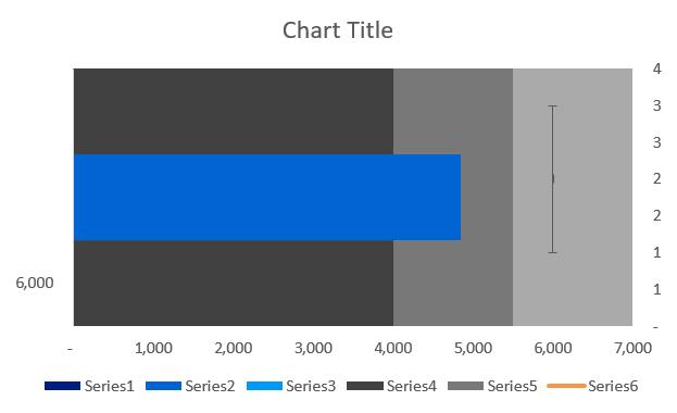
Now we will have the makings of a Target Bar:
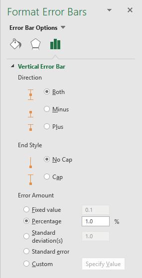
Select the Error bar and bring up the Chart ToolTips (CTRL + 1). Make sure the direction is set to ‘Both’, and that the ‘End Style’ is set to ‘No Cap’. Change the ‘Error Amount’ to 1.0%:
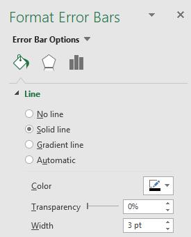
Move on to the ‘Fill & Line’ tab on the ToolTip. We set the width to 3pt and assigned a black colour to the bar.
Next steps:
- remove the y-axis and the legend
- rename the Chart Title and move it to the left side
- re-size the chart to accommodate for the Chart Title
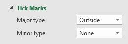
- add tick marks.
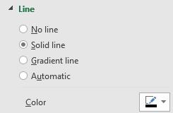
- give the x-axis a black line
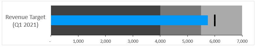
There we have it, a dynamic Bullet Chart!
With a revenue value of 5,750 the chart looks like:
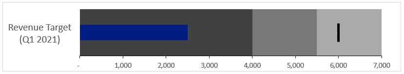
Revenue of 2,500:
Vertical Bar charts are similar but have a few differences:
- you need to use a Stacked Column chart
- the Series formula has inverted inputs =SERIES(,BC!$H$18,BC!$H$19,4)
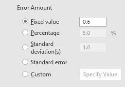
- use horizontal error bars (delete the vertical bar instead), and instead of setting the ‘Error Amount’ to a Percentage set it to a ‘Fixed value’ of 0.6.
We are good to go!
That’s it for this week. Check back next week for more Charts and Dashboards tips.