
Summing Else To Do
For sampling purposes, business unit summaries and many other reasons, sometimes you need to sum every Nth item in a list. But how do you do it? By Liam Bastick, director with SumProduct Pty Ltd.
Query
I have read other articles on finding the position of the Nth item (see Finding the Nth Item on a List), but my problem is slightly different.
I have a regular list of data and I need to sum every fourth item in the list. Is there a simple formulaic way I can perform this in Excel?
Advice
This is a common query in financial modelling as accountants and financial analysts often need to perform calculations on every other line, every third line, etc. In the specific question above the sum requires every fourth item, but I will show a generic technique that works for every Nth item instead.
We have introduced the MOD() function in a previous article (please see A Modicom of MOD for full details). That article mentions summing every Nth item using array functions (see Array of Light for more on array functions) in passing, so I thought I would give a fuller explanation using a non-array approach here, which will use less system memory here.
The MOD function, MOD(number,divisor), returns the remainder after the number (first argument) is divided by the divisor (second argument). The result has the same sign as the divisor.
For example, 9 / 4 = 2.25, or 2 remainder 1. MOD(9,4) is an alternative way of expressing this, and hence equals 1 also. Note that the 1 may be obtained from the first calculation by (2.25 – 2) x 4 = 1, i.e. in general:
MOD(n,d) = n – d*INT(n/d),
where INT() is the integer function in Excel.
We can use this function to help us with this problem. If we wish to sum every fourth item, then we want the fourth item, the eighth, the 12th, the 16th and so on, i.e. we sum when:
MOD(Row_Number,4)=0.
This means when the remainder when the Row_Number is divided by four is precisely zero. In general to sum every Nth item, we would sum when
MOD(Row_Number,N)=0.
Let’s consider the following example which comes from the attached Excel file:
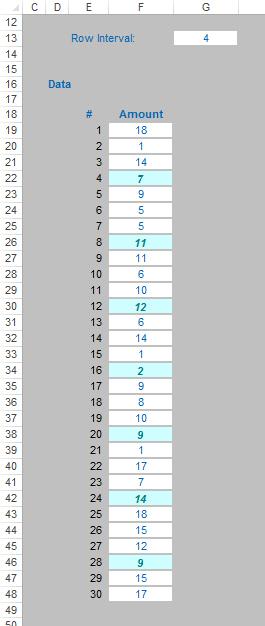
Here (using conditional formatting), I have highlighted every fourth item in the list.
I have the condition when to sum, just not the formula. To do this, let me remind you of another favourite. At first glance, SUMPRODUCT(vector1,vector2,…) appears quite humble. Before showing an example, though, look at the syntax carefully:
- A vector for Excel purposes is a collection of cells either one column wide or one row deep. For example, A1:A5 is a column vector, A1:E1 is a row vector, cell A1 is a unit vector and the range A1:E5 is not a vector (it is actually an array, but more on that later). The ranges must be contiguous; and
- This basis functionality uses the comma delimiter (,) to separate the arguments (vectors). Unlike most Excel functions, it is possible to use other delimiters, but this will be revisited shortly below.
Consider the following sales report:
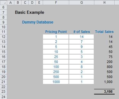
The sales in column H are simply the product of columns F and G, e.g. the formula in cell H12 is simply =F12*G12. Then, to calculate the entire amount cell H23 sums column H. This could all be performed much quicker using the following formula:
=SUMPRODUCT(F12:F21,G12:G21),
i.e. SUMPRODUCT does exactly what it says on the tin: it sums the individual products.
Where SUMPRODUCT comes into its own is when incorporating criteria. This is done by considering the properties of TRUE and FALSE in Excel, namely:
- TRUE*number = number (e.g. TRUE*4 = 4); and
- FALSE*number = 0 (e.g. FALSE*88=0).
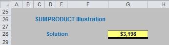
Returning to our example:
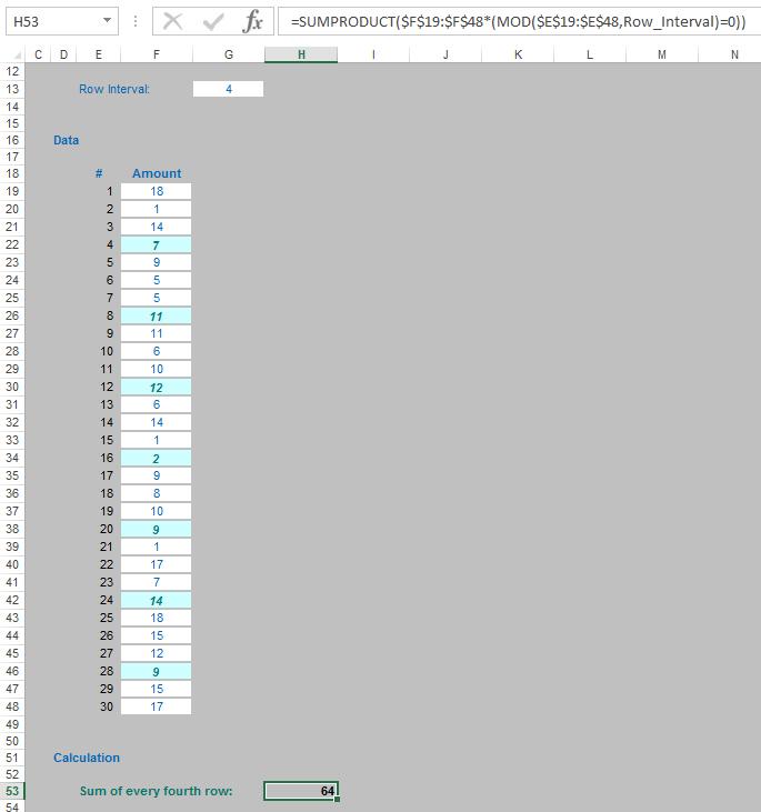
Cell H53 provides my suggested solution:
=SUMPRODUCT($F$19:$F$48*(MOD($E$19:$E$48,Row_Interval)=0)),
where Row_Interval is the named range (cell G13 in the example above).
SUMPRODUCT simply sums cells F19:F48 subject to the corresponding row number in column E being precisely divisible by the Row_Interval (in this case, 4), i.e. when a cell in the range E19:E48 satisfies the condition MOD(Cell_Value_in_Column_E,Row_Interval)=0.
Word to the Wise
As mentioned earlier, in a previous article we provided an array solution to this problem. SUMPRODUCT is often referred to as a “pseudo-array” function. Whilst it dispenses with the need to use an array formula, it behaves similarly to array formulae and therefore the range considered should not be any larger than necessary in order not to slow calculation performance any more than necessary.
If you have a query for this section, please feel free to drop Liam a line at liam.bastick@sumproduct.com or visit the website www.sumproduct.com