Finding the Nth Item on a List

Sometimes, first is not the be all and end all. Here, we look at locating duplicate matches in a list. By Liam Bastick, Director with SumProduct Pty Ltd.

Query

I am trying to find the position of the nth item in a list rather than the first necessarily. How do I do this?

Advice

Sometimes first is not always best. You might wish to locate the seventh item on an invoice or the third sister to attend school, etc. Presently, Excel has no standard function for this although the first match can be found easily using the MATCH function:

which returns the relative position of the first item in a list that (approximately) matches a specified value (see >Are Things LOOKing UP for INDEX and MATCH? for more details). It is not case sensitive (see Finding an EXACT Match for more details on case sensitive matching).

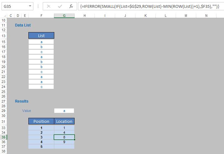
Let’s consider the following example which comes from the attached Excel file:

Imagine we wished to locate the position in the list of the third occurrence of the letter “a”. This occurs in row 22, which happens to be the eighth item in the list, i.e. the position is 8.

This calls for an array formula:

In this case, List would be the column vector F15:F24 and n would be 3, viz.

Arrays were discussed previously in Array of Light. Essentially, array formulae perform multiple calculations on one or more of the items in an array and are entered using CTRL + SHIFT + ENTER (the braces, “{” and “}” then appear, they cannot be typed in). Array formulae can return either multiple outputs or a single result. There are two types:

• Formulae that work with an array or series of data and aggregate it, typically using SUM(), AVERAGE(), MIN(), MAX() or COUNT(), to return a single value to a single cell. Microsoft calls these single cell array formulae.
• Formulae that return a result in to two or more cells (there are various formulae that will do this including MINVERSE(), LINEST() and TRANSPOSE()). These types of array formulas return an array of values as their result and are referred to as multi-cell array formulae.

The solution here is an example of a single cell array formula. It returns a single value after aggregating a range of data.

How it Works

To understand how this formula works, let’s look at the formula from inside to out starting with ROW(List)-MIN(ROW(List))+1. The ROW() function takes the row number so ROW(List)-MIN(ROW(List))+1 calculates the position of an element in List relative to the first item in the list (e.g. if the list started on row 1, then the second item on the list would be ROW(Row 2)-MIN(ROW(e.g. Row 1))+1) which would be 2-1+1 which equals 2.

IF(List=”a”,ROW(List)-MIN(ROW(List))+1) produces an array of positions which contain the letter “a”, i.e. {1,4,8,9} in our example list. It should be noted that it is commonplace in array IF() formulae not to specify what should happen if the condition is false (it is assumed the value is FALSE or nil).

The SMALL(List,n) function finds the nth smallest value in a list. Therefore, in our formula SMALL(IF(List=”a”,ROW(List)-MIN(ROW(List))+1),n) this finds the nth smallest item, so the third smallest value of {1,4,8,9} is 8.

Finally, IFERROR(SMALL(IF(List=”a”,ROW(List)-MIN(ROW(List))+1),n),”") uses IFERROR() to return “” (i.e. an empty cell) if we are looking for the nth item in the list where n is larger than the number of items in the list. This stops #NUM! being returned as a value and makes the formula ‘tidier’.

Since the formula considers a range of cells, this needs to be entered as an array formula – hence the braces.

Word to the Wise

If you want to find the nth value from the bottom up (instead of from the top down), use the LARGE() function instead of the SMALL() function.