LIFO Parole

I have twice previously considered modelling inventory, using both a simple averaging method to value the stock sold and then on a First In, First Out (FIFO) basis, which was a little bit trickier.  Since then, I have been inundated with people asking me to complete the set: how do you model on a Last In, First Out (LIFO) basis? 

There has been a little bit of naval gazing on this one (Pearl Harbo(u)r is my favo(u)rite) – not because I couldn’t produce an immediate solution, but that I tried to come up with a cleverermethod.  Well, truth is, dear reader, I failed.  Time to come clean.

Before anything, allow me to be clear here.  The LIFO method of inventory valuation is prohibited under International Financial Reporting Standards (IFRS), although it is permitted under the United States generally accepted accounting principles (US GAAP).

Why the controversy?  Potentially, LIFO may distort both the financial statements and financial analysis.  There are several ways this can be allowed to happen.  For example:

• assuming inventory costs increase over time, LIFO can understate a company's earnings for the purposes of keeping taxable income low
• the inventory valuation reported may be outdated, spoiled, expired or else obsolete
• in a liquidation scenario, earnings may be inflated artificially by selling off inventory with seemingly low carrying costs.

So do bear this all in mind before you start modelling this way!  You might get “LIFO parole” if judged.

Having stepped off my sanctimonious soapbox, let’s consider an example (available in the attached Excel file):

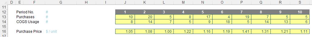
I shall jump to precisely what the problem is here.  Can you provide me with the formula for deriving the costs of the inventory in Period 6?  The problem is I can only reduce the requirement by four [4] given the inventory procured in the same period, but I am unsure what my stock levels are remaining for the items purchased in previous periods for different prices.

Algorithmically, I can figure it out:

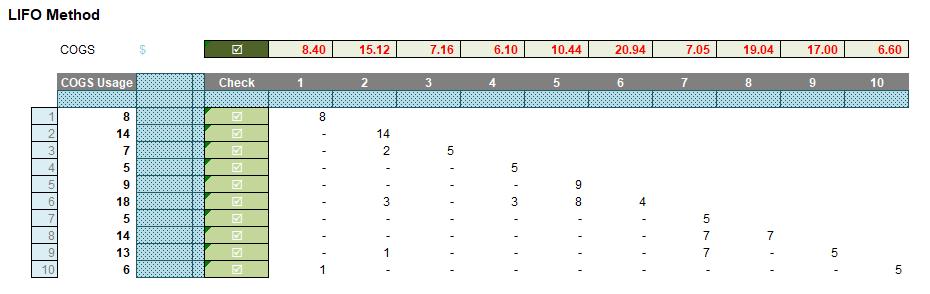
• In Period 1, I purchase 10, sell eight [8], for $8.40 (8 x $1.05) and have two remaining
• In Period 2, I purchase 20 and sell 14.  As I have sold less or equal to the number purchased, the LIFO cost is easy, I just calculate 14 x $1.08 which gives me $15.12.  I am left with two remaining still from Period 1 and six in Period 2
• In Period 3, I purchase five [5] but sell seven [7].  Therefore, the first five sold are easy to cost (5 x $1.00) but I have to check the remainder for the previous period, which there are sufficient (six), so the remaining three may be calculated (2 x $1.08), giving me a total cost of $7.16.  I am left with two still from Period 1, four from Period 2 and none remaining in Period 3
• In Period 4, I purchase eight [8] but only sell five [5], so the costing is easy again, being (5 x $1.22, which is) $6.10.  This leaves remaining inventory of two from Period 1, four from Period 2 and three from Period 4
• Period 5 works along the same lines.  Since the purchases (17) exceed the sales (9), my costs are trivial being (9 x $1.16, which equals) $10.44.  This leaves remaining inventory of two from Period 1, four from Period 2, three from Period 4 and eight from Period 5
• Finally, we get to Period 6.  We only procured four [4], but we sold 18.  The first four items are easy to cost (4 x $1.19), but the remaining 14 need to be sourced.  Eight will come from Period 5 (8 x $1.16), three will come from Period 4 (3 x $1.22) and the remaining three from Period 2 (3 x $1.08).  This will be a total cost of $20.94, leaving two remaining from Period 1 and one from Period 2.

See how awkward this is getting and the fact we are having to keep a running total of remaining inventory levels by period?  It is easy when the number of items used is less than or equal to the total items bought.  The issue is when we have to raid the cupboard for older supplies.  We need to know what is remaining and that depends upon what was used last period.  However, that period’s data depends upon what was used the period prior to that.  And so on.  This is an example of recursion and recursive formulae require Excel’s latest wunderkind LAMBDA.  That takes me back (groan – Ed.).  Given this function is not available in all versions of Excel, I shall not be exploring that option here.

Therefore, unlike solutions for weighted average costing and First In, First Out (FIFO) methods, I shall have to fall back on what is known as a grid calculation.  I have been unable to construct a shortcut approach that will bypass this recursion.  For those who fail to see the distinction between the other methods and the LIFO scenario, whilst it’s true that both the weighted average and the FIFO methods required data from the previous period, they only needed aggregated totals; here, we have to keep tabs on what stock remains and in which period it was purchased, i.e. an ever-increasing array of values.  Excel’s in-cell calculations using “traditional, long served” functions do not appear to assist in this instance.

To be clear, not for a moment am I stating unequivocally there isn’t some shortcut technique, it’s just as at the time of writing, I haven’t thought of one (and I have even started to get imaginative with some of the lesser-known financial functions to try and concoct some Machiavellian approach).  Alas, so far, it has eluded me.

Therefore, let’s consider the grid approach:

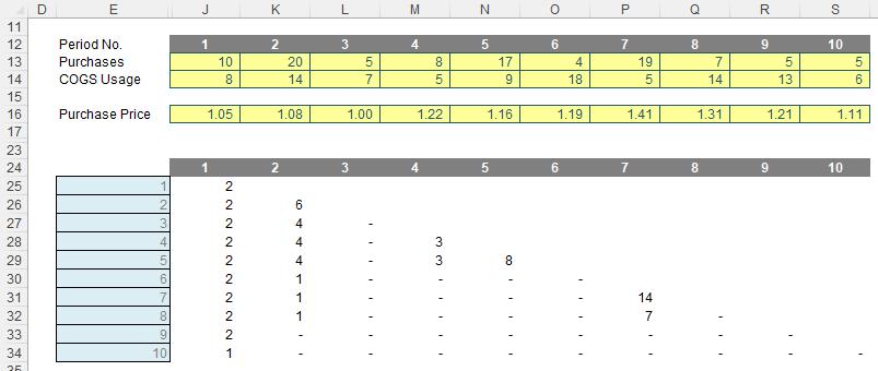
Do the values in rows 25:30 of the graphic look familiar?  This is keeping a running total of what inventory still remains.  As explained above, this is essential for working out costing and also useful for working out the age or remaining inventory, possible stockouts, etc.

In order to derive these numbers, I used a favourite function of mine…

Refresher on OFFSET

It seems every other article I bring this old chestnut up!  The syntax for OFFSET is as follows:

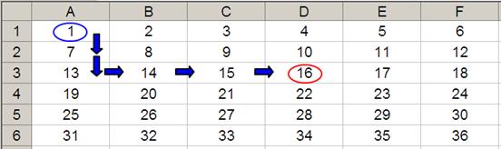
The arguments in square brackets (height and width) may be omitted from the formula, but I will need them here.  In its most basic form, OFFSET(reference, x, y) will select a reference x rows down (-x would be xrows up) and y columns to the right (-y would be y columns to the left) of the reference reference.  For example, consider the following grid:

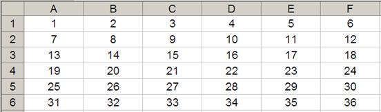
OFFSET(A1,2,3) would take us two rows down and three columns across to cell D3.  Therefore, OFFSET(A1,2,3) = 16, viz.

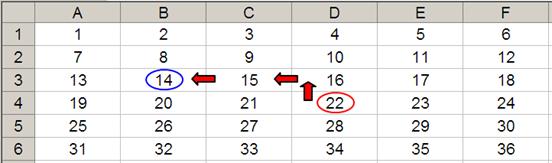
OFFSET(D4,-1,-2) would take us one row up and two rows to the left to cell B3.  Therefore, OFFSET(D4,-1,-2) = 14, viz.

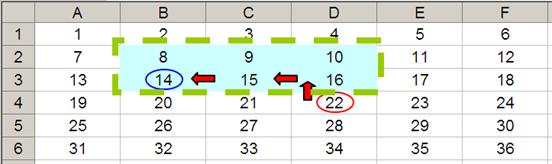
OFFSET may also take advantage of the height and width arguments.  If we extend the above formula to OFFSET(D4,-1,-2,-2,3), it would again take us to cell B3, but then we would select a range based on the height and width parameters.  The height would be two rows going up the sheet, with row 14 as the base (i.e. rows 13 and 14), and the width would be three columns going from left to right, with column B as the base (i.e. columns B, C and D). 

Hence, OFFSET(D4,-1,-2,-2,3) would select the range B2:D3,viz.

Note that OFFSET(D4,-1,-2,-2,3)= #VALUE! where dynamic arrays are not recognised, since Excel cannot display a matrix in one cell, but it does recognise it.  However, if after typing in OFFSET(D4,-1,-2,-2,3) we press CTRL + SHIFT + ENTER, we turn the formula into an array formula: {OFFSET(D4,-1,-2,-2,3)} (do not type the braces in, they will appear automatically as part of the Excel syntax).  This gives a value of 8, which is the value in the top left-hand corner of the matrix, but Excel is storing more than that.  This can be seen as follows:

• SUM(OFFSET(D4,-1,-2,-2,3)) = 72 (i.e. SUM(B2:D3))
• AVERAGE(OFFSET(D4,-1,-2,-2,3)) = 12 (i.e. AVERAGE(B2:D3)).

SUM(OFFSET) and OFFSET will both be useful here.

Returning to LIFO

Let’s revisit the grid:

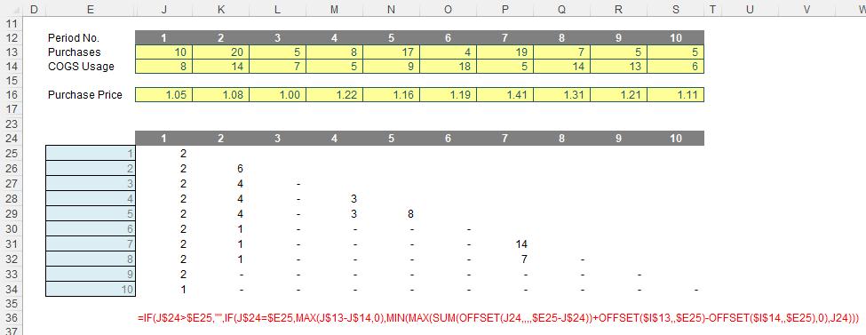
The formula in cell J25 is

Lovely.  I think this needs to be broken down!

Note that row 24 and the cells E25:E34 both denote the period number, so for eight periods we would have an eight by eight grid, and here, we have a 10 by 10 matrix.  Clearly, I cannot have any remaining inventory relating to periods later than the period presently being analysed, e.g. for Period 3, I could not take into account stock to be purchased in Period 4 or subsequently.  This rules out half of my matrix.  The formula

considers this.  If the period number to be analysed is greater than the period of usage the formula returns empty data (“”)."the period of usage the formula returns empty data (“”).  So far, so good.  The next period to consider is the actual period items are purchased and used (i.e. the leading diagonal of the grid), when the period number in the row and column are equal:

In this situation, the remaining stock would be given by any excess of purchases over COGS usage, so for cell J25 this would equate to MAX(J$13-J$14,0).  The restriction is so that this number may not go negative.  It’s a simple calculation.  The issue is what follows!

Here, I have constructed a formula that is both replicable and scalable (this is why I have needed the OFFSET function). 

Given the recursive nature of the calculation, perhaps starting in Period 1 is not ideal as this situation cannot occur (this calculation only comes into force when we are looking to use prior period inventory to service current year usage – in the first period, by definition, we will have no prior inventory in this example).

Therefore, it is probably more appropriate to consider the copied down formula in cell J26 instead:

Let’s first consider the difference between the purchases made in Period 2 (cell K13, 20) and the COGS usage (cell K14, 14).  This would be given by the formula

Now the problem here is I want to copy this formula across the row so that it always references these cells:

That’s OK, but when I copy the formula down a row I also need it to anchor to rows 13 and 14 respectively:

However, on the next row down I will want to reference rows L13-L14,etc.  I would have to write a different formula each row, which would become cumbersome: imagine coding a 20-year monthly model.  No thank you.  This is why I use

This uses the cell before the first purchased amount and the first used amount and then moves one column across for every row of the table (so Period 1 will use column J, Period 2 will use column K, etc.).  This now makes sense.

Whilst this formula seems long this is now keeping track of the surplus or deficit of the purchases with regard to the COGS usage for the current period.  I write it this way round so that if it is in deficit it will be negative.  Let me park this part of the calculation for a second.

Allow me to now consider

This formula considers the cell directly above the cell in question (so here it references J25 as the formula is in cell J26).  It doesn’t move any rows or columns and the height / depth is not defined (so it will just be the current row) but the width is given by the formula $E26-J$24, i.e. the current period number less the period number of the inventory being considered.  Therefore, for cell J26, the width would be the current period (2) less the period the inventory in question was acquired (1), which would be 2 – 1 = 1.  Thus, SUM(OFFSET(J25,,,,$E26-J$24)) is equivalent to =SUM(J25). 

That seems convoluted.

But let’s take the formula in cell K30 instead (the formula relating to inventory acquired in Period 2 but considered in Period 6):

The relevant part of the formula here would be

Here, the width would be the current period (6) less the period the inventory in question was acquired (2), which would be 6 – 2 = 4.  Thus, SUM(OFFSET(K29,,,,$E30-K$24)) is equivalent to =SUM(K29:N29).  Similarly, the relevant part of the formula in cell L30 would be =SUM(L29:N29)and the formula in cell M30 would be =SUM(M29:N29).

This is a cumulative sum in reverse and has the same effect as putting the formula

in cell N30 and copying itright to left.  The advantage of using the SUM(OFFSET) formula is you may copy it down and across the entire matrix: it is repeatable and scalable, even if it is unintelligible!

Thus, returning to our original formula in cell J25,

this formula sums all the past inventory available acquired from that inventory period onwards that is still available (this is why it refers to the previous row) and adds any current period surplus / deducts any current period deficit.

If there is a deficit, the sum of the prior periods’ inventory will be reduced (and indeed, could become negative).  This is not possible, so we need to restrict the sum:

However, if this value is non-zero, it is possible the surplus could exceed the inventory for this period previously calculated.  That is clearly incorrect, so we must restrict the value to be no greater than the prior period balance for the period in question, viz.

This effectively calculates which inventory is utilised on a LIFO basis to cover any deficit and is clearly demonstrated in the grid.  Putting it all together, we obtain our original monster calculation:

This wouldn’t be as horrible if we modified the formula for each row, but written this way, the matrix may be increased seamlessly.

Now we have the remaining inventory profile, calculating the COGS for the period is relatively simple with the assistance of the SUMPRODUCT function.  And yes, I know, it must be at least four minutes since I last mentioned this function…

Refresher on SUMPRODUCT

Consider the following example:

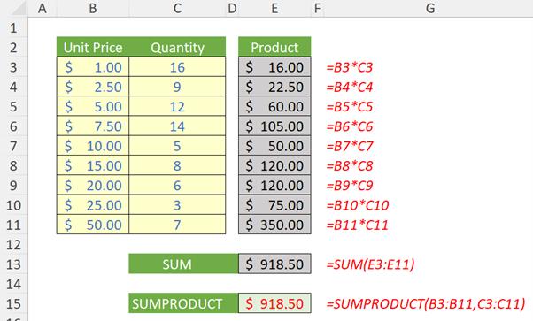
Here, I have various pricing points and the corresponding quantities sold.  To calculate my total sales, I can compute my sales by taking the product of Unit Price multiplied by Quantity on a line by line level and then summing them.  As you can see, SUMPRODUCT does it all in one go:

Here, I will combine it with OFFSET…

Calculating COGS

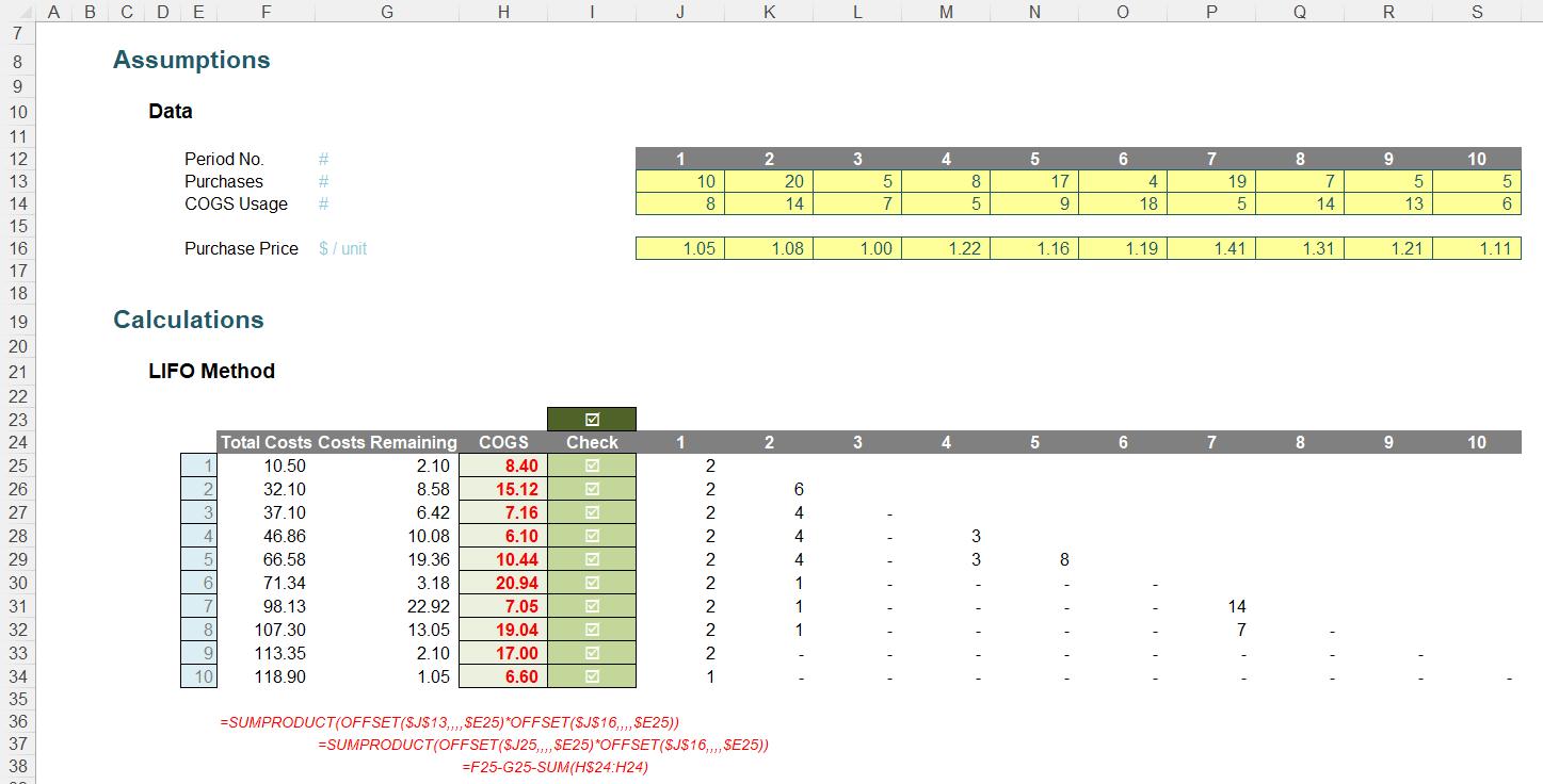
The formula in cell F25 calculates the Total Costs and is given by

You are probably starting to understand these formulae now.  This formula takes the Purchases (row 13) and multiplies them by the Purchase Price (row 16), before summing the total.  The width of the range extends by one period each time, e.g.

etc.

This clearly gives the total purchase cost up to and including the period in question.

Similarly, the formula for Costs Remaining in cell G25 is given by

This is very clearly a similar idea, except it cross-multiplies the relevant purchase prices by the inventory remaining at that point in time.

The difference between these two amounts is the Total COGS for all periods.  Therefore, to determine the costs for the current period only the formula for COGS (in cell H25) is given by

At last!  A simple formula!  This calculation subtracts the Costs Remaining from the Total Costs (F25-G25) and then deducts the total COGS for previous periods (SUM(H$24:H24) – referring to text is merely treated as zero courtesy of the SUM formula) to leave us with the COGS for the current period.

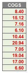
The COGS are then cited in column H:

As I explained earlier, I would have liked to have found a simpler non-grid approach, but the LIFO method requires a recursive algorithm.  Nevertheless, I am happy to challenge my readers to construct an alternative approach that doesn’t involve LAMBDA.

Word to the Wise

Apologies, it’s not the simplest concept we have ever discussed, but this is one of the most commonly requested problems I receive in financial modelling these days.  Do watch out though: it is prohibited in many accounting jurisdictions.

In the attached Excel file, I also include an alternative approach, which calculates the COGS costs directly in the matrix instead.  I do not go through the methodology here, but it employs a similar technique.  Have fun reviewing it!