
Historical vs. Actual vs. Forecast
Liam Bastick, director (and Excel MVP) with SumProduct Pty Ltd, highlights some of the common issues and scenarios in financial modelling / Excel spreadsheeting. This time he looks at how to create formulae which consider historical, actual and forecast data simultaneously.
Many accountants and analysts have to analyse trends using past and current performance in order to create informed forecasts for the future. This requires three distinct datasets:
- Historical information: data that has now been gathered that actually happened. This is often recorded in Management Information Systems, general ledgers, tax returns, etc. This data tends to have one thing in common: it’s a matter of fact
- Actual data: whilst historical information summarises past data that has been locked down, “actuals” may be slightly more fluid in that data may be available for the first nine months of the year (say) combined with three months’ projections, based upon predicted orders, work schedules, hours of operation and so on
- Forecast projections: these numbers are usually based upon calculations and correlations with the historical / actual data. The first two datasets may be distinct and independent, but typically, there is a relationship with at least one of the other types and forecast projections.
You may or may not agree with my above summation. That’s not really the point here. They key takeaway here is that when we undertake financial modelling, we often have more than one situation that occurs over the time periods, e.g.

The problem with data set out like this is two-fold:
- Less experienced modellers will use three types of data entry for the three segments, which may be a combination of formulae and / or hard code. The concern is someone else will come along and copy one formula across the entire row which will not be appropriate for the other data categories
- More experienced modellers acknowledge one consistent formula must be used across the row – but then try and do all calculations in the one cell and construct a formula that typically starts =IF(IF(… etc.
Neither is optimal, but the second option is nearer the truth. The problem with =IF(IF(… is it intimidates end users who try to follow it, with a succession of nested calculations. Excel 2016’s IFS function is even worse as people have to understand both the concept of nesting and the prevailing syntax. Stepping out seems way simpler.
I am going to take start with an example with three scenarios:
- Historical: in my example, these will be inputs, but they could link to another file (say)
- Actual: in my example, again, these will be inputs, but this could be a calculation based on actual data for the period to date and then extrapolated (say)
- Forecast: in my example, this will be a formula.
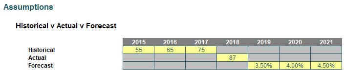
You could have five situations, two linked, one hard coded and two formulaic – the idea would remain the same. The first thing is to collate all necessary inputs:
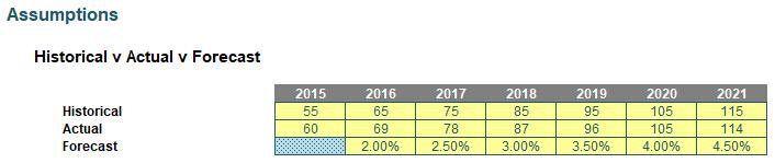
My plan here is to use the first row of data for historical periods, the second row for the actual period, and then use the growth rate on the previous period for forecasts. Clearly, only one value would be used in each year (column).
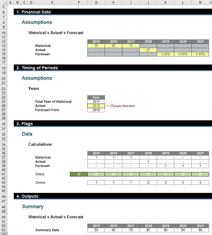
Next, I created a selector for which year was the actual year:
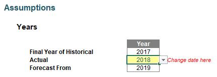
The input cell (Actual, in yellow) drives the other two dates, as Historical would have to be all periods up to the year before and Forecast from the following year. With more situations, there would have to be more inputs, but the general idea would remain similar.
I can now create a “flag” system (1 for on / yes, 0 for off / no) to denote which situation relates to which period:
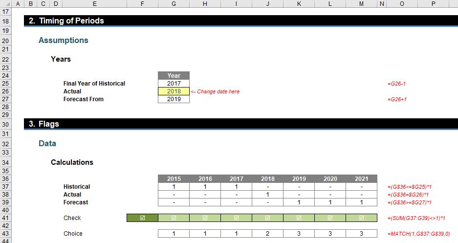
The Historical flags (row 37 of the image above) are 1 for years 2015, 2016 and 2017 using the formula
=(G$36<=$G25)*1
in cell G37, for example. This checks that the years in question is less than the value in cell G25, which is 2017. Similarly, the Actual formula is
=(G$36=$G26)*1
and the Forecast formula is
=(G$36>=$G27)*1
which means all formulae are simple.
A check has been put in row 41 to ensure there is a ‘1’ (but only one ‘1’) in each column (year) too:
=(SUM(G37:G39)<>1)*1
Finally, the Choice (row 43) uses the MATCH function (see >Are Things LOOKing Up for INDEX and MATCH? for more information) to determine where the 1 in each column is, i.e. 1 if it is in the first row, 2 if it is in the second, etc.
=MATCH(1,G$37:G$39,0)
MATCH(lookup_value,lookup_array,[match_type]) returns the relative position of an item in an array that (approximately) matches a specified value. It is not case sensitive.
The third argument, match_type, does not have to be entered, but for most situations, I strongly recommend that it is specified. It allows one of three values:
- match_type 1 [default if omitted]: finds the largest value less than or equal to the lookup_value – but the lookup_array must be in strict ascending order, limiting flexibility;
- match_type 0: probably the most useful setting, MATCH will find the position of the first value that matches lookup_value exactly. The lookup_array can have data in any order and even allows duplicates; and
- match type -1: finds the smallest value greater than or equal to the lookup_value – but the lookup_array must be in strict descending order, again limiting flexibility.
When using MATCH, if there is no (approximate) match, #N/A is returned (this may also occur if data is not correctly sorted depending upon match_type).
For example:
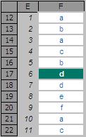
In the figure above, MATCH(“d”,F12:F22,0) gives a value of 6, being the relative position of the first ‘d’ in the range. Note that having match_type 0 here is important. The data contains duplicates and is not sorted alphanumerically. Consequently, match_types 1 and -1 would give the wrong answer: 7 and #N/A respectively.
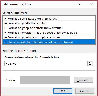
Returning to the 1’s and 0’s section (the latter displayed as dashes in the graphic), these values have also been used to drive conditional formatting in the original input section too, viz.
To create grey cells, I have simply highlighted the entire range and use conditional formatting (in the ‘Styles’ section of the ‘Home’ tab of the Ribbon, ALT + O + D) as follows:
We are pretty much done now. All that is needed is a formula for the output:
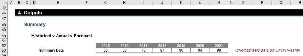
The formula
=CHOOSE(G$43,G$13,G$14,F53*(1+G$15))
in cell G53 uses the value in row 13 if the choice is 1 (historical selected), in row 14 if the choice is 2 (actual) and multiplies the previous period by 1 plus the growth rate in row 15 if the choice is 3 (forecast) using the CHOOSE function.
The CHOOSE function employs the following syntax to operate:
CHOOSE(index_number, value1, [value2])
As a reminder, the CHOOSE function has the following arguments:
- index_number: this is required and is used to specify which value argument is to be selected. The index_number must be a number between 1 and 254, or a formula or reference to a cell containing a number between 1 and 254.
- if index_number is 1, CHOOSE returns value1; if it is 2, CHOOSE returns value2; and so on
- if index_number is less than 1 or greater than the number of the last value in the list, CHOOSE returns the #VALUE! error value
- if index_number is a fraction, it is truncated to the lowest integer before being used.
- value1, value2, ...: value 1 is required, but subsequent values are optional. There may be between 1 and 254 value arguments from which CHOOSE selects a value or an action to perform based on index_number. The arguments can be numbers, cell references, defined names, formulas, functions, or text.
You can find out more about CHOOSE at Do You Choose to Use CHOOSE?.
The great thing about this method is regardless of whether end users know about conditional formatting, INDEX or CHOOSE, the actual final calculation is easy to follow on paper, viz.
And that’s what financial modelling is all about! You can check out our example file here.
If you have a query for the Thought section, please feel free to drop Liam a line at liam.bastick@sumproduct.com or visit the SumProduct website.