Getting a Date if You’re a Modeller…

Wondered why it text so long to get a date in the modelling industry? We figure out why, by modelling. By Liam Bastick, director (and Excel MVP) with SumProduct Pty Ltd.

Query

When I download data into Excel, I’m having real problems in turning the dates imported into dates that Excel will recognise.  Do you have any advice?

Advice

[Before I am inundated with emails suggesting that COM add-ins Power Query and Power Pivot can help on occasion, this is not a solution for everyone, so I am going to ignore their existence here.]

Sometimes, when data is imported from third party software, reported dates are not identified as such by Excel.  This is for two reasons:

1. Many dates in third party software are stored as text strings, such as “25 December 2016”, “25/12/16”, “Nigel” and so on.
2. Dates in Excel are stored as numbers.  On a PC, 1 January 1900 is day 1, 2 January 1900 is day 2 and so on.  These numbers are known as serial numbers.  Excel cannot always detect a relationship between a text string (which typically has a numerical value of zero or cannot be evaluated) and the corresponding serial number.

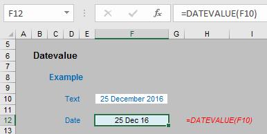
On some occasions, the date may be converted to a serial number (and then formatted as a date) by simply multiplying by 1 (this is a common trick for numbers in general stored as text).  If this does not work, you can always try the DATEVALUE function which converts dates stored as text to dates stored as values, viz.

DATEVALUE function

Sometimes it is more painful though and you need to resort to Excel’s text functions that manipulate more testing text strings.  I have covered these before (see the Text Messages Thought article for more details), but in summary the most common functions in this category include:

• LEN(Text) gives the length of Text in terms of number of text characters
• LEFT(Text,n) returns the first n characters (reading from left to right of the text string referenced)
• RIGHT(Text,n) which returns the last n characters (reading from right to left of the text string referenced).  Similar to LEFT(Text,n), non-numerical values will remain non-numeric and values of n greater than the referenced text string itself will merely return the entire text string
• MID(Text,Start_Number,n) is like a halfway house between LEFT() and RIGHT().  This function returns n characters from the referenced text string starting with the character in position Start_Number.  Again, truncated text will not become numerical by default and if n exceeds the number of characters from Start_Number to the final character, the remaining characters are displayed rather than an error value
• FIND(Find_Text,Within_Text,[Start_Number]) is a search function which is case sensitive but does not allow wildcard characters.  It seeks out the first instance of a character or characters (typed in inverted commas) in the Within_Text text string.  The Start_Number argument is optional (hence the square brackets in the syntax) so that the first few characters in a text string may be ignored.  If the Find_Text cannot be located within Within_Text the error #VALUE! is returned
• SEARCH(Find_Text,Within_Text,[Start_Number]) is a search function which is not case sensitive but does allow for wildcard characters (wildcards will be discussed in next month’s article).  It seeks out the first instance of a character or characters (typed in inverted commas) in the Within_Text text string.  The Start_Number argument is optional (hence the square brackets in the syntax) so that the first few characters in a text string may be ignored.  If the Find_Text cannot be located within Within_Text the error #VALUE! is returned
• TRIM(Text) simply removes superfluous spaces within a text string, e.g. “John     Smith     ” would become “John Smith” instead.

I now construct a comprehensive example to show how you might get a date from a particularly horrible text string.  And yes, before anyone writes in, there may be many different solutions to my illustration below.  However, I choose the following approach to showcase many of the text functions described above.

Comprehensive Example

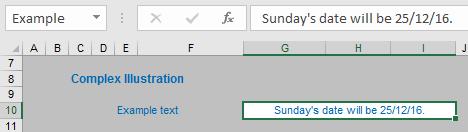
Consider the following example:

DATEVALUE function

This is a bit messy for several reasons:

• The date is embedded in the text
• Presumably other dates in the list will have different lengths, e.g. “Wednesday’s date will be 28/12/16.” will have more characters in the text string and therefore have the date positioned later in the text string
• In this example it is assumed days and months only have the number of characters required, e.g. September will be “/9/” rather than “/09/”.  This means that the number of characters that need to be extracted to formulate the day and month needs to be a variable number (either one or two).

Therefore, I need to develop an approach that will take these issues into account. 

I am going to break this down into three key elements, namely obtaining the day, the month and finally the year.  Let’s go get that day number first.

To show you how I develop my logic, feel free to download the attached Excel file or follow along with the images:

Obtaining the day number

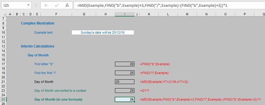
First of all, I need to locate a unique character that always occurs a set number of characters before the beginning of the date element.  The letter “b” meets this criterion.  No matter which day of the week is selected the first appearance of the letter “b” will always occur three characters before the start of the date.  To find this character, I use the formula

where Example is the cell reference containing the text string (G10 in the example above).  In this instance, the letter “b” occurs in position 20 of the text string “Sunday’s date will be 25/12/16.”  This means that the date will start in position =FIND("b",Example)+3, i.e. in position 23.

I need to address the fact that the day number may be one or two characters long.  A simple way to determine this is using the formula

noting that FIND locates the first occurrence of a character or set of characters in a text string.  The first “/” is situated in position 25 of our Example.  Since our date starts in position 23 and the first “/” is in position 25, this means the day number must be in positions 23 and 24, i.e. it is a text string containing two, rather than one, characters.  
In our example above, with the formula for locating “b” in cell I17 and the formula for locating “/” in cell I19, the day number may be extracted using the computation

It should be noted that although this formula correctly returns the value “25” being the day number it is left aligned.  It is important that you notice this.  It means that that this is a text value rather than a numerical value.  This may cause problems for us yet, so we need to multiply this result by one to convert it to a number.  Therefore, if we remove all of the cell references and put all of the calculations in one ‘megaformula’ we get the following in cell I25 of our illustration:

It looks horrible but it gets us the day number.  This approach of replacing the cell reference with the underlying formula is known in modelling as the Principle of Staggered Development.  This is how longer formulae should be constructed – safely.

It’s now time to turn our attention to the month number.

Obtaining the month number

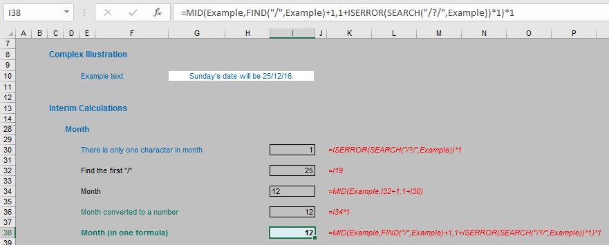
I already know where the first “/” is situated from above (position 25), so I know that the month number starts in position 26.  My problem is, I don’t know whether the month number contains one character (e.g. 1, 2, 3) or two (e.g. 10, 11, 12).  This is where the formula in cell I30 comes in:

Unlike FIND, SEARCH is not case sensitive but it does allow wildcards and ? is a very useful wildcard.  The difference between * and ? is that the latter only allows for one character, so the formula above is searching for “/?/”, i.e. only one character between the two obliques.  If it can find this, SEARCH returns the value, ISERROR will return the value FALSE and FALSE*1 is zero.  If it cannot find this string – that is, there are two characters in the month number – SEARCH will return an error, ISERROR will return the value TRUE and TRUE*1 is one (do you know your TRUE times tables?).  In summary, the formula in cell I30 will return the value:

• 0 if the month number contains only one character
• 1 if the month number contains two characters.

Therefore, the month may be derived from the formula in cell I34:

Ensuring the result is a number and substituting the cell references with the appropriate formula, I obtain my second ‘megaformula’:

Next, it’s time to get the year.

Obtaining the year number

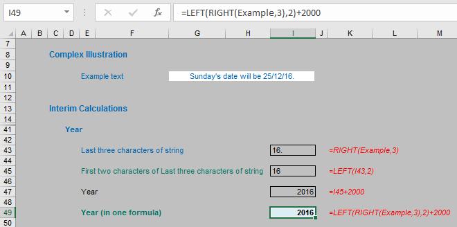
That’s fairly straightforward because the two digits always occur in the third from last and second from last positions of the Example text string (since the full stop is the last character in the illustration).

The graphic (above) shows the step through in deriving the formula in cell I49, but I think it is reasonably straightforward to go straight to it:

The RIGHT inner formula extracts the last three characters and LEFT then takes the first two letters of this abridged text string.  Adding 2,000 automatically ensures Excel treats the resulting text string as a value.  That’s a nice trick to keep up your sleeve for safekeeping.

Finally, we just need to put it all together:

Putting it all together

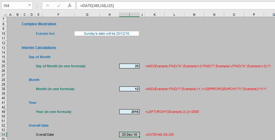
With the day number in cell I25, the month number in cell I38 and the year in cell I49, the DATE(Year,Month,Day) function can combine the results into a date using the formula

That is deceptively simple, but once you replace the cell references with the underlying calculations it looks a little more complex:

Now that may not be pretty but it is pretty effective.

As I stated earlier, you may come up with alternative ideas to get to the same result.  That’s fine.  All I intended to do here was construct an example to demonstrate where and how to use which text function when and why.

Word to the Wise

Our comprehensive example spawned a monster this time.  It is long, not exactly transparent and contains hard code.  This is far from “Best Practice”.  Unfortunately, sometimes in modelling – like in life – the means justifies the end and I am a hypocrite.  All rules have exceptions.  Except this one.

(Don’t think about it too much!)

Want to read more on modelling with dates? Here is an article that details how to build a model that forecasts on the weekly basis. If you have any questions please feel free to drop Liam a line at liam.bastick@sumproduct.com.