First and Last and Always

So you need to interpolate between two data points, which may not always occur at the same points and / or intervals.  Here’s some practical tips by Liam Bastick, Managing Director (and Excel MVP) with SumProduct Pty Ltd.

Let’s imagine you have prepared a set of reporting dates and the known amounts presented at irregular reporting dates:

Requirement Excerpt

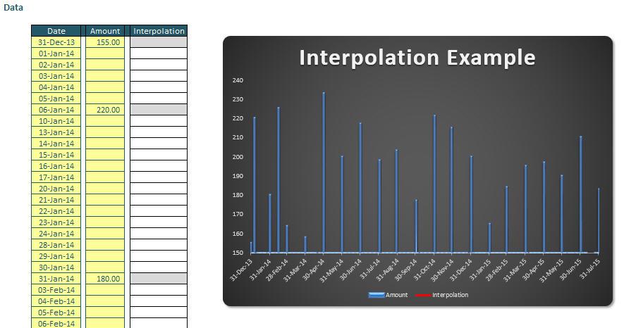
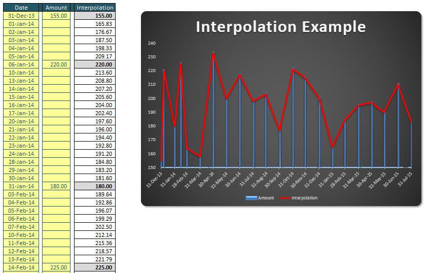
The challenge here is to create one unique formula that can be copied down a column to linearly interpolate based on the number of days, viz.

Illustration

The conditions are:

• There should only be one unique formula, copied down the column
• No array (CTRL + SHIFT + ENTER) formulae allowed
• No macros or user-defined functions.

The reason for this is purely because of its practical implications.  For those working in finance, often projections will be made periodically, but not necessarily for every date under scrutiny.  Therefore, you need to identify an “on-track” value with each date to identify significant variances quickly.

Assuming a straight-line method of projection, this approach to predicting values between two points is known as linear interpolation.  Consider the following example:

Linear Interpolation

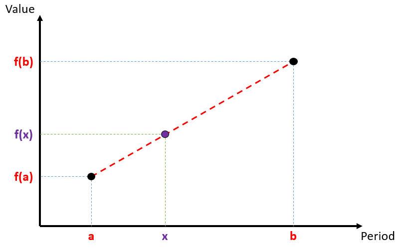
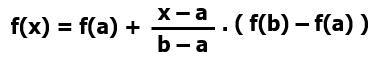
If a and b are points in time (say) and f(a) and f(b) are their corresponding values, then the linearly interpolated output of x (where a ? x ? b), f(x), is given by the equation

This is all we need to create our formula, with x as our date and f(x) the corresponding value.  All we need to determine are the following:

• The date of the last value actually input (a)
• The value of the last value actually input (f(a))
• The date of the next value actually input (b)
• The value of the next value actually input (f(b)).

Before you all write in and tell me I am over-complicating matters, I want to demonstrate how to look up both the next and last values in a table as these are important tricks in financial modelling in their own right.  

In our example, our problem was made more difficult in that any cell in the input data table could have a value entered so we needed to treat a and b as variables.  This requires us to use three functions: INDEX, MATCH and LOOKUP.

INDEX and MATCH have been discussed before (please see >this article for more details), but unbelievably, I haven’t yet discussed LOOKUP.  I had better put that right now!

Aside: Introducing LOOKUP (if there’s anyone out there that doesn’t know it…)

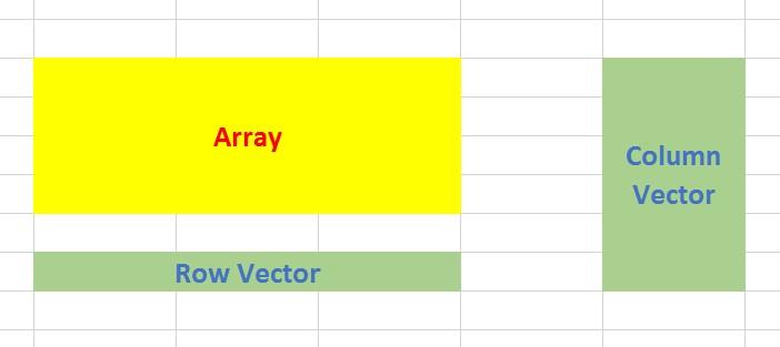
LOOKUP is quite useful for modelling.  It has two forms: an array form and a vector form.  I suppose I had better explain the jargon:

• An array is a collection of cells consisting of at least two rows and at least two columns
• A vector is a collection of cells across just one row (row vector) or down just one column (column vector).

The diagram should be self-explanatory:

Arrays and Vectors

The array form of LOOKUP looks in the first row or column of an array for the specified value and returns a value from the same position in the last row or column of the same array:

where:

• lookup_value is the value that LOOKUP searches for in an array.  The lookup_value argument can be a number, text, a logical value, or a name or reference that refers to a value
• array is the range of cells that contains text, numbers, or logical values that you want to compare with lookup_value.

The array form of LOOKUP is very similar to the HLOOKUP and VLOOKUP functions.  The difference is that HLOOKUP searches for the value of lookup_value in the first row, VLOOKUP searches in the first column, and LOOKUP searches according to the dimensions of array.

If array covers an area that is wider than it is tall (i.e. it has more columns than rows), LOOKUP searches for the value of lookup_value in the first row and returns the result from the last row.  Otherwise, LOOKUP searches for the value of lookup_value in the first column and returns the result from the last column instead.

The alternative form is the vector form:

The LOOKUP function vector form syntax has the following arguments:

• lookup_value is the value that LOOKUP searches for in the first vector
• lookup_vector is the range that contains only one row or one column
• [result_vector] is optional – if ignored, lookup_vector is used – this is the where the result will come from and must contain the same number of cells as the lookup_vector.

Like the default versions of HLOOKUP and VLOOKUP, lookup_value must be located in a range of strictly ascending values, i.e. where each value is larger than the one before and there are no duplicates.

Let me demonstrate with the following example (the full set of examples may be found in the attached Excel LOOKUP file):

Example

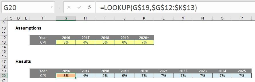
Imagine you have an annual model forecasting for many years into the future.  Creating inputs will be time consuming if data has to be entered on a period by period basis.  But there is a shortcut.

Do you see the data table in cells F12:K13 above?  The value in the final cell of the first row is actually “2020” not “2020+”.  It appears that way due to custom number formatting (CTRL + 1):

Format Cells

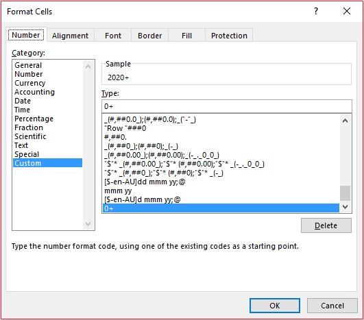
The syntax “0+” adds a plus sign to the number although Excel still reads the value as 2020. 

The formula uses the array version of LOOKUP, looking up the year in the first row of the data tabe and returning the corresponding value from the final row.  When a year is selected which is greater than 2020, the 2020 value is used as LOOKUP seeks out the largest value less than or equal to the value sought.  Therefore, we don’t need to have lengthy data tables – once we assume inputs will be constant thereafter, we can just curtail the input section.

Using the array form of LOOKUP is dangerous though.  What if someone accidentally inserts rows?  The lookup will “flip” to look the first and last columns instead, which is not what is required. Using the vector form is safer:

Example (Continued)

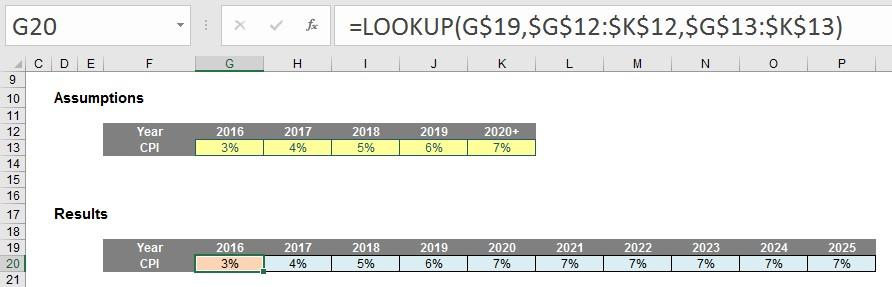
Whilst the formula contains one more argument, the formula is more stable.  Further, the lookup_vector and the result_vector do not need to be in the same worksheet or even the same workbook.  In fact, as long as there are the same number of elements in each, one can be a row vector and the other a column vector.

LOOKUP is very useful when the lookup_vector contains data in strict ascending order.  Where do we find this?  Dates in time series – LOOKUP is very useful for financial modelling / forecasting.  Just be careful though; consider the following scenario:

Example (Continued)

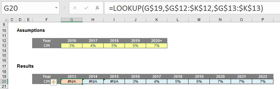
Here, the same formula generates an #N/A error.  This is because the date is smaller than the smallest value in the data range.  LOOKUP is not quite clever enough to use the first value unprompted, but a simple tweak of the formula will suffice:

Example (Continued)

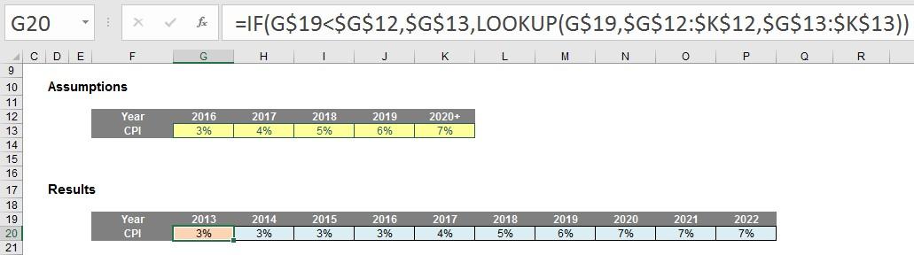
Here, the formula has been modified to:

The added IF statement checks to see if the year is smaller than the first year in the data table and if so, returns the first result.  Simple!

It is with this final modification – in its vector form – that I usually use LOOKUP to return values for certain time periods where I do not want to have an input for each period modelled. Very useful!

Back to the Problem…

To recap, if a and b are points in time (say) and f(a) and f(b) are their corresponding values, then the linearly interpolated output of x (where a ? x ? b), f(x), is given by the equation

As stated above, we need to determine the following:

• The date of the last value actually input (a)
• The value of the last value actually input (f(a))
• The date of the next value actually input (b)
• The value of the next value actually input (f(b)).

Let me explain how to get the values.

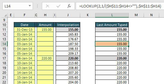
The value of the last value actually input (f(a))

Perhaps this is the most awkward formula to understand.  The formula is given by:

In our example (see Attached Excel Example Solution File):

Finding the Last Value Actually Input

So how does this work?

I thought it was obvious (!).  The 1/(Range<>””) portion returns an array that contains a 1 (TRUE) or 0 (FALSE) value only for each cell in the Range, depending on whether that cell is blank or not.

The next step is to use the 1 or 0 values as the Denominator in 1/Denominator. This calculates the inverse value, and you end up with either 1 (1/1) or a #DIV/0! error (1/0).  Since the value being searched for in the array is the value 2 – and does not exist – the LOOKUP function actually ignores all the error values in the array, returning the last array element that contains a 1 value instead. This corresponds to the last cell in the Range that is non-blank.

Who’s for “Blah, blah, blah, just use this formula when you need it”..?

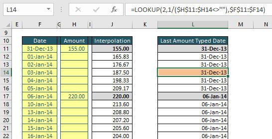
The date of the last value actually input (a)

This is actually simply a modified version of the above formula using the LOOKUP formula with two ranges, viz.

In our example (see Attached Excel Example Solution File):

Finding the Last Date Where Data Was Actually Input

Next!

The value of the next value actually input (f(b))

As mentioned above, we have explained INDEX and MATCH before, but the idea is similar to the above LOOKUP formula:

This gives the next non-blank value in the Remaining_Range.  Note the extract INDEX(Remaining_Range=””,) – this provides another array, this time of TRUE’s (where values are blank) and FALSE’s otherwise.  MATCH simply returns the position of the first occurrence.

In our example (see Attached Excel Example Solution File):

Finding the Next Value Actually Input

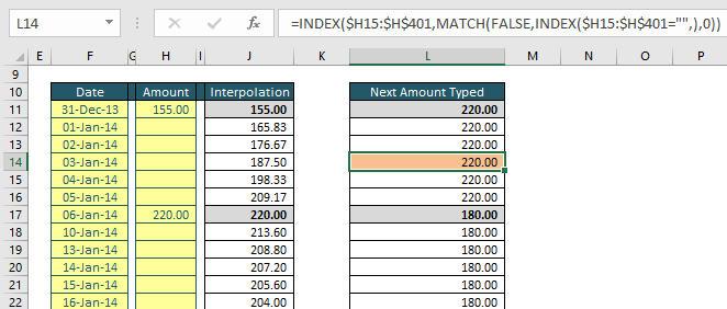
which leaves us with…

The date of the next value actually input (b)

This is actually simply a modified version of the above formula using the INDEX MATCH INDEX formula with two ranges, viz.

In our example (see Attached Excel Example Solution File):

Finding the Next Date Where Data Was Actually Input

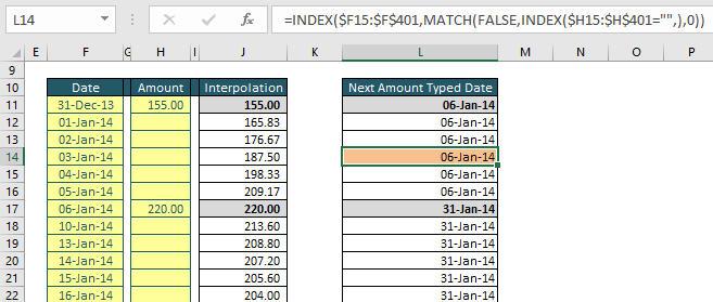
Voila!

Suggested Solution

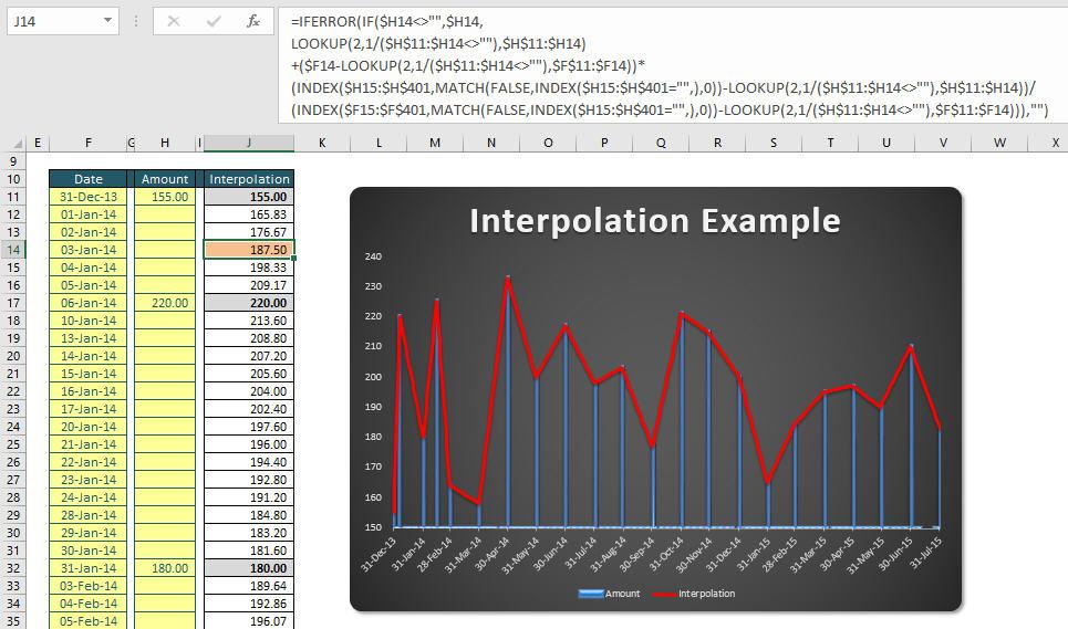
That’s it.  We just need to put all of these formulae into the master computation

This leads to the following – deep breath! – horror formula in cell F14 of our Attached Excel Example Solution File:

All I have added are two checks:

1. Use the value input when it appears
2. Make the cell blank if it gives rise to an error.

Suggested Solution

Er, simple!

If you have more questions on the VLOOKUP or LOOKUP, you can find another thought article on it here, otherwise please feel free to drop Liam a line at liam.bastick@sumproduct.com