
Dynamic Arrays: One Year On
16 September 2019
It’s 12 months since Microsoft rocked the calculation boat with its new range of dynamic array functions and features. Those of us lucky enough to get it in Excel Insider Fast raved incessantly. But what’s actually happened one year later..? We take a look.
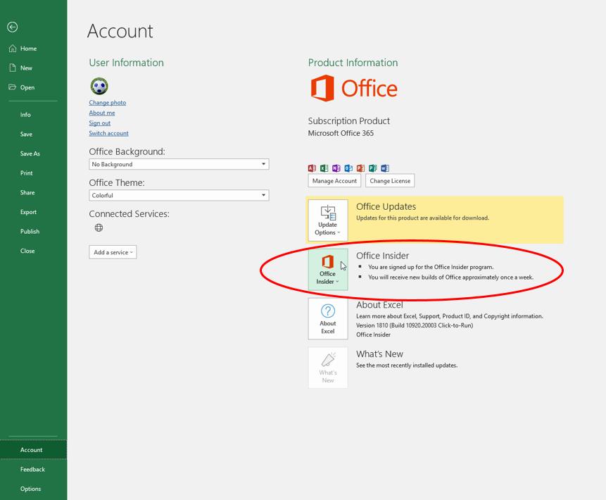
365 days later and dynamic arrays are still in “Preview” mode, i.e. it’s not yet “Generally Available” but it has moved into all of Office 365 Insider Fast and some of Insider Slow and Monthly Targeted (version 1906 Builds 11901.20080 and later). You can register for Insider in File -> Account -> Office Insider in Excel’s backstage area.
The world has now realised that it won’t be coming to the perpetual licence versions such as Excel 2016 and Excel 2019. That wasn’t immediately clear, but users have come to realise this. It’s not so much that it has been in Preview for so long – we get that the calculations are revolutionary and there are still issues to work out such as:
- being able to have totals at the bottom of spilled arrays
- allowing spilled arrays to accept formatting
- having calculations generate the same results if calculated in a different order (see below).
It’s the fixation with Office 365 only that worries me. Whilst this helps the clamour for the subscription model, this may be a mistake. Modellers are going to be loathe to use functions and features that the majority of end users will not be able to take advantage of. It may mean adoption will be slow for features people should be using in their millions. Similar judgment calls were made with Power Pivot, and eventually, Microsoft relented and made it available to all in Windows versions of Excel. I can’t help but think a similar perspective should be taken here.
Currently, we therefore have two types of Excel:
- DA Excel: Excel that supports dynamic arrays, its functions and features
- Legacy Excel: the “traditional” Excel that is still wrapped in the world of CTRL + SHIFT + ENTER and does not support dynamic arrays.
This leads to compatibility issues.
Compatibility Issue #1: @ and SINGLE
You may recall the SINGLE function that was released last year.
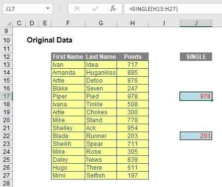
In the past, if you entered =A$1:A$10 anywhere in rows 1 through 10, the formula would return only the value from that row. In DA Excel, typing this formula would create a Spilled Array Formula. To protect existing formulae, the SINGLE function was created to return a single value using logic known as implicit intersection. SINGLE may return a value, single cell range or an error:
=SINGLE(value)
For example, the two SINGLE formulae here are supplied a range, H13:H27, and return the values in cells H17 and H22 respectively, corresponding to the rows that were held in common:
Later, after its initial release, SINGLE was replaced with @ as follows:
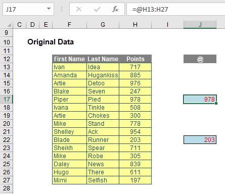
Now, I mention this history with good reason. Excel will only remove @ from a formula where previous Excel versions would have used implicit intersection (as described above) to return a single value from a range, a named range or function parameter.
On the positive side, if you attempt to enter such a formula, Excel will warn you and do its utmost to stop you. It is still possible to cause an issue though. For example, in DA Excel, you could create the following formula:
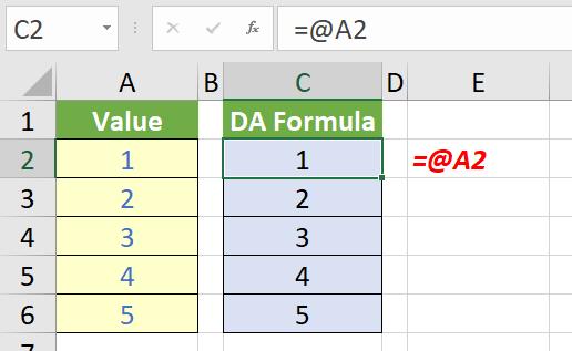
In Legacy Excel, this would appear as:
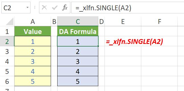
Notice the error message is =_xlfn.SINGLE(A2), not =_xlfn.@(A2). This is confusing if you don’t know the history of the @ operator. Worse comes if you try to evaluate this formula:
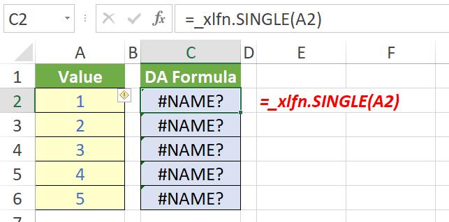
It generates an #NAME? error, which is far from ideal.
Compatibility Issue #2: Spill References
A formulaic reference to an entire dynamic array may use the spill reference suffix operator (that’s a mouthful), e.g.
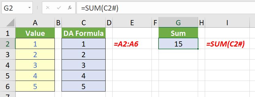
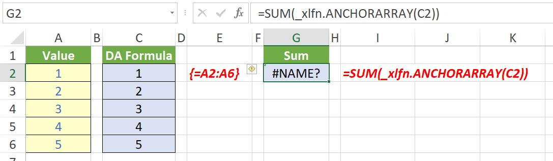
The formula =SUM(C2#) sums the entire spilled range emanating from cell C2. Unfortunately, this is not converted as you might hope in Legacy Excel:
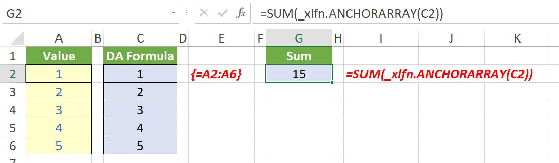
The formula in cell G2 is now =SUM(_xlfn.ANCHORARRAY(C2)) and, again, will not evaluate, viz.
Compatibility Issue #3: Uninvited CTRL + SHIFT + ENTER (CSE) Array Formulae
Take another look at that last example:
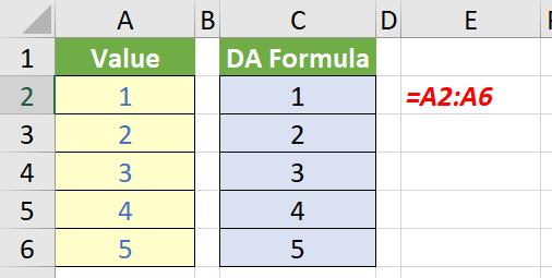
In DA Excel, the formulae in cells C2:C6 contain the spilled formula =A2:A6. In Legacy Excel, these formulae have been replaced as follows:
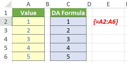
The formula {=A2:A6} (created by using CTRL + SHIFT + ENTER) has been entered in each cell in cells C2:C6. This is because any formula that DA Excel thinks could return an an array (even if it is actually only returning a single value) is converted to a CTRL + SHIFT + ENTER (CSE) array formula in previous versions. This can impact memory and is creating unnecessarily complex formulae. This can cause several issues:
- a single vell containing a non-spilling formula is made unnecessarily complex and may not evaluate correctly
- a DA Excel dynamic array formula that is either spilling or blocked (#SPILL!) will be converted to a fixed CSE formula in earlier versions of Excel
- a formula entered in DA Excel as a multi-cell CSE formula may have backward compatibility issues.
You need to take great care when working with such instances.
Another Issue: Calculation Order Concern
There is another problem that is an issue in DA Excel. When I calculate something in Excel, if I use the same formula, I must get the same answer, right? Well – not necessarily. Consider the following:
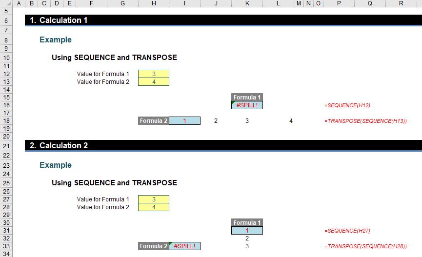
In the example above, Calculations 1 and 2 are identical but deliver different results (i.e. different #SPILL! errors). Why?
- In Calculations 1 and 2, both values for Formula 1 and Formula 2 were originally set to 1. This causes no #SPILL! errors
- In Calculation 1, the value for Formula 2 (cell H13) was then changed to 4 with no error
- Then, in Calculation 1, the value for Formula 1 (cell H12) was changed to 3. This caused the resultant #SPILL! error in cell K16
- Next, in Calculation 2, the value for Formula 1 (cell H27) was changed to 3 with no error
- Then, in Calculation 2, the value for Formula 2 (cell H28) was changed to 4. This caused the resultant #SPILL! error in cell I33.
I am not sure what the solution is for this problem. Technically, #SPILL! is working correctly, but it doesn’t seem right that two results may be generated in this instance depending upon what input I change first. The jury remains out on this one.
Not All Gloom and Doom
RANDARRAY is one of the original functions in DA Excel. Because it’s not yet Generally Available, it’s had a facelift in the last six months. This is an important thing to note – this was the first time ever a function had been released publicly by Microsoft and then had its syntax changed. This is something that is possible to do before a function or feature becomes Generally Available – “Preview” means Microsoft reserves the right to change something as they see fit. That’s a good thing here.
Originally, the RANDARRAY function returned an array of random numbers between 0 and 1. However, there was a general sense of underwhelm with this function and the new and improved version has just been released. It now allows you to set you own maximum and minimum and decide whether you want the values returned to be decimals (e.g. 17.4381672…) or integers (whole numbers).
The new syntax for the function is now as follows:
=RANDARRAY([rows], [columns], [min], [max], [integer])
The function has five arguments, all supposedly optional (but upon testing, we weren’t quite as convinced):
- rows: this specifies how many rows the results should spill over. If omitted, the default value is 1
- columns: this specifies how many columns the results should spill over. If omitted, the default value is also 1
- min: this is the minimum value that may be selected randomly. If this is not specified, it is assumed to be zero (0)
- max: this is the maximum value that may be selected randomly. If this is not specified, it is assumed to be 1
- integer: if this is set to TRUE, only integer outputs are allowed; the default value (FALSE) provides non-integer (decimal) results.
Other points to note:
- if rows or columns refers to a blank cell reference, this will generate the new #CALC! error
- if rows or columns are entered as decimals, the values used will be truncated to the number before the decimal point (e.g. 3.99 will be treated as 3)
- if rows or columns is a value less than 1, #CALC! will be returned
- if integer is set to TRUE and either min or max is not an integer, this will generate an #VALUE! error
- max must be greater than or equal to min, else the error #VALUE! is returned.
When we originally discussed the RANDARRAY function, we used this rather comprehensive example to create a list of random integers between two values:
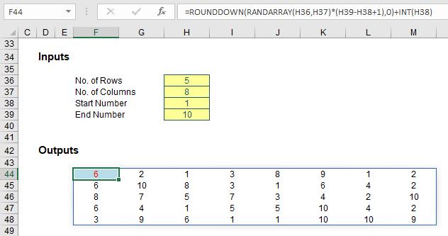
Originally, the formula in cell F44 was
=ROUNDDOWN(RANDARRAY(H36,H37)*(H39-H38+1),0)+INT(H38)
and my past article explained how this worked. However, it’s much easier now:
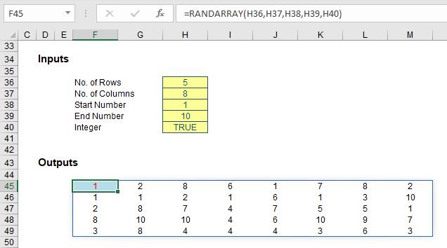
The “new improved” formula in cell F45 (it’s moved down a row due to the additional argument required in cell H40) is simply
=RANDARRAY(H36,H37,H38,H39,H40)
This is much simpler – and pretty cool.
Impact of XLOOKUP and XMATCH
Since the announcement of dynamic arrays, there has been another major announcement of two new functions, XLOOKUP and XMATCH. At the time of writing, these two functions are both in Preview mode in Office 365 Insider Fast only.
XLOOKUP has the following syntax:
XLOOKUP(lookup_value, lookup_vector, results_array, [match_mode], [search_mode])
On first glance, it looks like it has too many arguments, but often you will only use the first three:
- lookup_value: this is required and defines what value you want to look up
- lookup_vector: this reference is required and is the row or column of data you are referencing to look up lookup_value
- results_array: this is where the corresponding item is you wish to return and is also required (even if it is the same as lookup_vector). This does not have to be a vector (i.e. one row or one column of cells): it may be an array (with at least two rows and at least two columns of cells). The only stipulation is that the number of rows / columns must equal the number of rows / columns in the column / row vector – but more on that later
- match_mode: this argument is optional. There are four choices:
- 0: exact match (default)
- -1: exact match or else the largest value less than or equal to lookup_value
- 1: exact match or else smallest value greater than or equal to lookup_value
- 2: wildcard match. You should use the special character ? to match any character and * to match any run of characters.
- search_mode: this argument is also optional. There are again four choices:
- 1: search first to last (default)
- -1: search last to first
- 2: what is known as a binary search, first to last (requires lookup_vector to be sorted). Just so you know, a binary search is a search algorithm that finds the position of a target value within a sorted array. A binary search compares the target value to the middle element of the array. If they are not equal, the half in which the target cannot lie is eliminated and the search continues on the remaining half, again taking the middle element to compare to the target value, and repeating this until the target value is found
- -2: another binary search, this time last to first (and again, this requires lookup_vector to be sorted).
XLOOKUP is a powerful substitute for both VLOOKUP and INDEX MATCH:
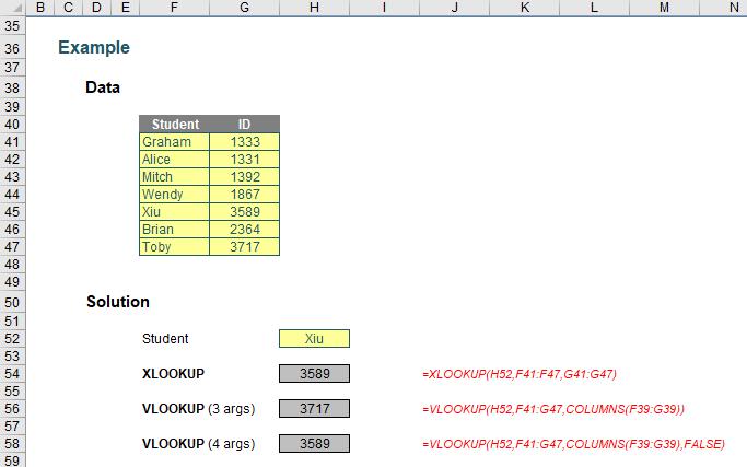
You can clearly see the XLOOKUP function is shorter:
=XLOOKUP(H52,F41:F47,G41:G47)
Only the first three arguments are needed, whereas VLOOKUP requires both a fourth argument, and, for full flexibility, the COLUMNS function as well. XLOOKUP will automatically update if rows / columns are inserted or deleted. It’s just simpler.
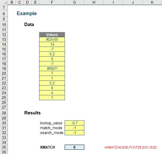
Further, the sister function XMATCH has the following syntax:
XMATCH(lookup_value, lookup_vector, [match_mode], [search_mode])
where:
- lookup_value: this is required and defines what value you want to look up
- lookup_vector: this reference is required and is the row or column of data you are referencing to look up lookup_value
- match_mode: this argument is optional. There are four choices:
- 0: exact match (default)
- -1: exact match or else the largest value less than or equal to lookup_value
- 1: exact match or else smallest value greater than or equal to lookup_value
- 2: wildcard match. You should use the special character ? to match any character and * to match any run of characters.
- search_mode: this argument is also optional. There are again four choices:
- 1: search first to last (default)
- -1: search last to first
- 2: this is a binary search, first to last (requires lookup_vector to be sorted)
- -2: another binary search, this time last to first (and again, this requires lookup_vector to be sorted).
As you can see, it’s a fairly straightforward addition to the MATCH family. It acts similarly to MATCH – just with heaps more functionality.
It’s clear to see both of these functions would work well with dynamic arrays and spilled references. Since the announcement of these two formulae, people have been knocking down the door to use them in a Generally Available environment.
Word to the Wise
I know no more than you, dear reader, but I have an inkling that Microsoft might be changing things up shortly. Dynamic arrays were publicly announced at Microsoft Ignite last year. This same conference is to be held in Florida in early November this year. I can’t help thinking…