
Automating a Table of Contents
This article shows you how to create a Navigation page in double-quick time. By Liam Bastick, Director with SumProduct Pty Ltd.
Query
I notice many of your example files come with a ready-made Table of Contents, which makes the workbook easier to navigate. Is there a quick way to create one of these?
Advice
Tables of Contents are a great way to navigate a workbook. If you have a central worksheet which contains hyperlinks to all other relevant sections, this means the modeller and end user alike are only ever two clicks away from somewhere else in the workbook.
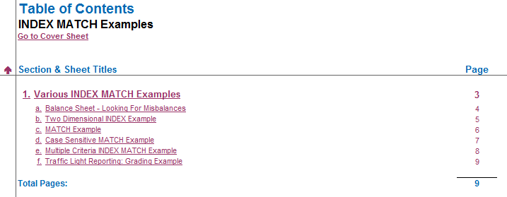
Table of Contents (such as the example above) can be created using various third party software, manually using hyperlinks (see Hyperlinking Chart Sheets for example), or else quickly and easily using a simple Visual Basic for Applications (VBA) macro.
I tend to use macros sparingly. There are some compatibility issues between versions of Excel, they can make models slower, less transparent and difficult to edit. However, there is a time and a place for most things and a very simple macro will provide a very simple Table of Contents in less time than it takes to read the end of this very long sentence.
I have discussed macros before (please see also Locating Links #2 ), but I will recap a couple of important points.
Checking Excel’s Security Settings
Because macros may execute all sorts of nasty code, Excel’s default setting is set so that macros will not run automatically. To ensure the macro below will work, you will first need to check / amend Excel’s security settings, viz.
Excel 2003 and earlier
- Call up the ‘Options’ dialog box (Tools -> Options or ALT + T + O);
- Select the ‘Security’ tab;
- In the ‘Macro security’ section, click on the ‘Macro Security…’ button;
- Ideally, select / confirm the setting as ‘Medium’. This means you can choose whether or not to run macros; and
- Excel may have to be closed and re-opened for these changes to be adopted
Excel 2007 and later
- Click on the Office Button;
- Click on ‘Excel Options’ (ALT + T + O is the equivalent of these first two steps);
- Select ‘Trust Center’ from the left hand columnar list;
- In the ‘Microsoft Office Excel Trust Center’ section, click on the ‘Trust Center Settings…’ button;
- Select ‘Macro Settings’ from the left hand columnar list (if the ‘Developer’ tab is displayed on the Ribbon, ALT + L + AS will get you to this point immediately); and
- In the ‘Macro Settings’ section, select ‘Enable all macros’ (note this is a slightly more dangerous option than its Excel 2003 counterpart)
Saving a File Containing Macros
For readers using Excel 2007 and subsequent versions, be careful when saving this file. It is safest to use the ‘Save As…’ option:
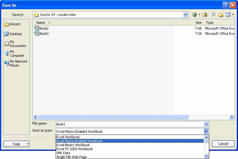
The default ‘Save as type:’ setting for Excel 2007 onwards is ‘Excel Workbook’, but this is a macro-disabled (and moreover, removed) setting. To retain the macro in the saved file, ensure that either the ‘Excel Macro-Enabled Workbook’ or, for better compatibility with earlier incarnations of Excel, ‘Excel 97-2003 Workbook’ type is selected.
How to Create a Simple Table of Contents
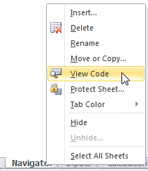
With the code provided below, simply add a worksheet called ‘Navigator’ (this name can be changed by amending the code). Then, right click on the ‘Navigator’ worksheet tab and select ‘View Code’, viz.
This will launch the Visual Basic Editor:
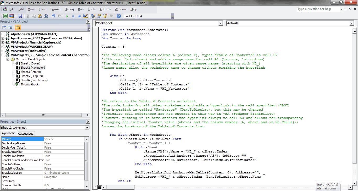
Not all of the above panes may be visible, but in the right hand pane (headed “Worksheet, Activate”) paste in the following code (as shown in the graphic above):
Private Sub Worksheet_Activate()
Dim wSheet As Worksheet
Dim Counter As Long
Counter = 8
'The following code clears column 6 (column F), types "Table of Contents" in cell C7
'(7th row, 3rd column) and adds a range name for cell A1 (1st row, 1st column)
'The destination of all hyperlinks are given range names (starting with HL_)
'Range names allow the worksheet name to change without breaking the hyperlink
With Me
.Columns(6).ClearContents
.Cells(7, 3) = "Table of Contents"
.Cells(1, 1).Name = "HL_Navigator"
End With
'Me refers to the Table of Contents worksheet
'The code looks for all other worksheets and adds a hyperlink in the cell specified ("A3")
'The hyperlink is called "Navigator" (TextToDisplay), but this may be changed
'Typically cell references are not entered in this way in VBA (reduced flexibility)
'However, putting it in here anchors the hyperlink always to cell A3 and allows for transparency
'Changing the initial Counter value (above) and the column number (6, above and in Me.Cells())
'moves the location of the Table of Contents list
For Each wSheet In Worksheets
If wSheet.Name <> Me.Name Then
Counter = Counter + 1
With wSheet
.Range("A3").Name = "HL_" & wSheet.Index
.Hyperlinks.Add Anchor:=.Range("A3"), Address:="", _
SubAddress:="HL_Navigator", TextToDisplay:="Navigator"
End With
Me.Hyperlinks.Add Anchor:=Me.Cells(Counter, 6), Address:="", _
SubAddress:="HL_" & wSheet.Index, TextToDisplay:=wSheet.Name
End If
Next wSheet
End Sub
That’s it. The code is not actually that long; I have added comments (which start with an apostrophe and wil appear in green, when pasted into the Visual Basic Editor) which should hopefully explain the rudimentary mechanics / logic of the procedure – and more importantly – how to customise it.
To assist, I have also provided an attached Excel file to demonstrate how this might work. Essentially, as worksheets are added, deleted, copied or moved, the Table of Contents will update displaying the new order of worksheets excluding the Navigator worksheet. The descriptions used will be derived from the worksheet tab names (so make your tab names descriptive!). It also adds a hyperlink on each worksheet (in cell A3 using the default code) back to the Navigator worksheet.
The macro runs every time either the worksheet is selected or a hyperlink is activated taking the user back to the Table of Contents.
One Last Thing
Readers may also note the worksheet titles displayed in cell A1 of each worksheet of the attached Excel file. The titles in my simple illustrative workbook reflect the workbook tab name using similar logic to the formula derived to list the workbook name (for consistency) described in Automated File Names.
It all comes together, you know!