Power Query: Top Two

Welcome to our Power Query blog. This week, I look at splitting my data into the top two (for example) and the rest.

I have some data from my imaginary salespeople that I used in Power Query: Group Functions.

This time, I want to give the commission total for 2019 to my two top salespeople, and then show an average for everyone else.

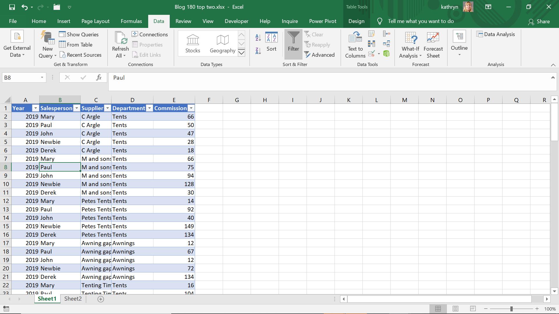
I start by extracting my data into Power Query, by using ‘From Table’ in the ‘Get & Transform’ section of the Data tab.

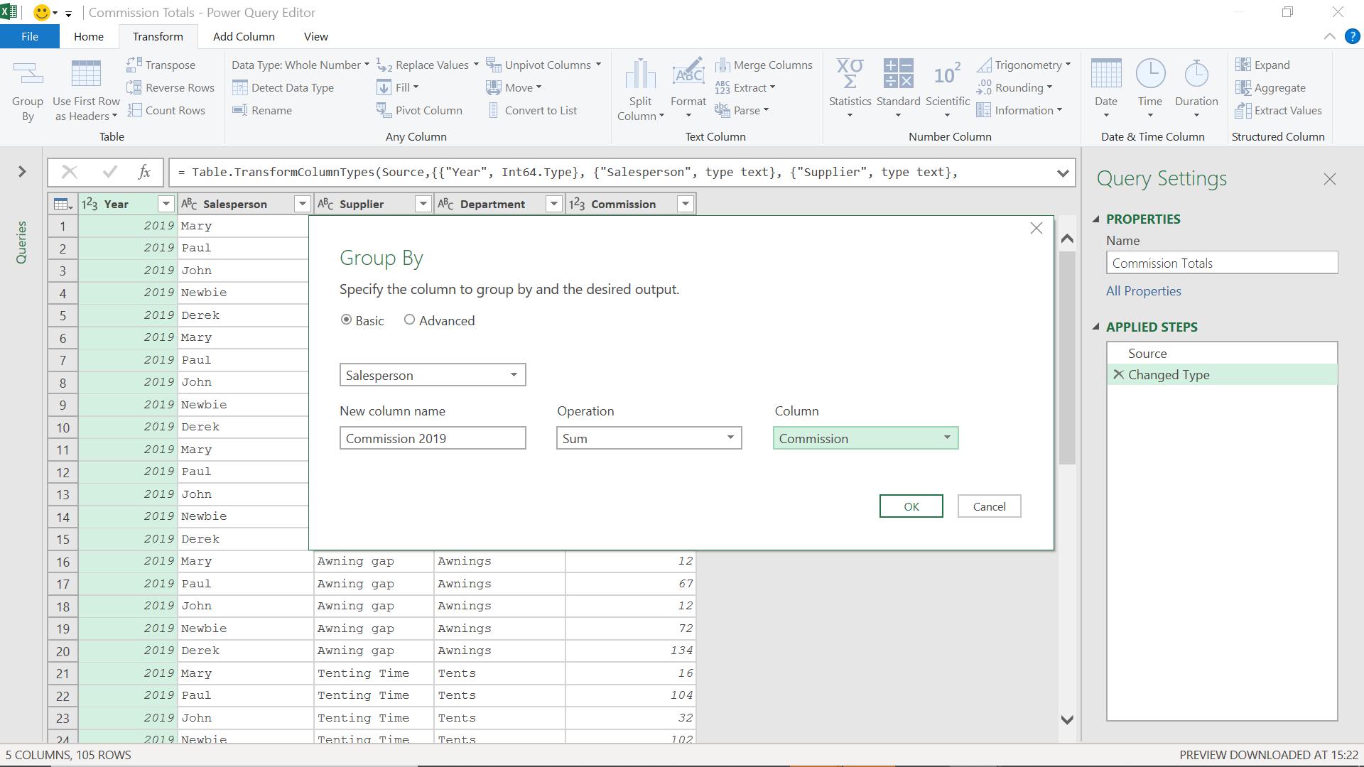
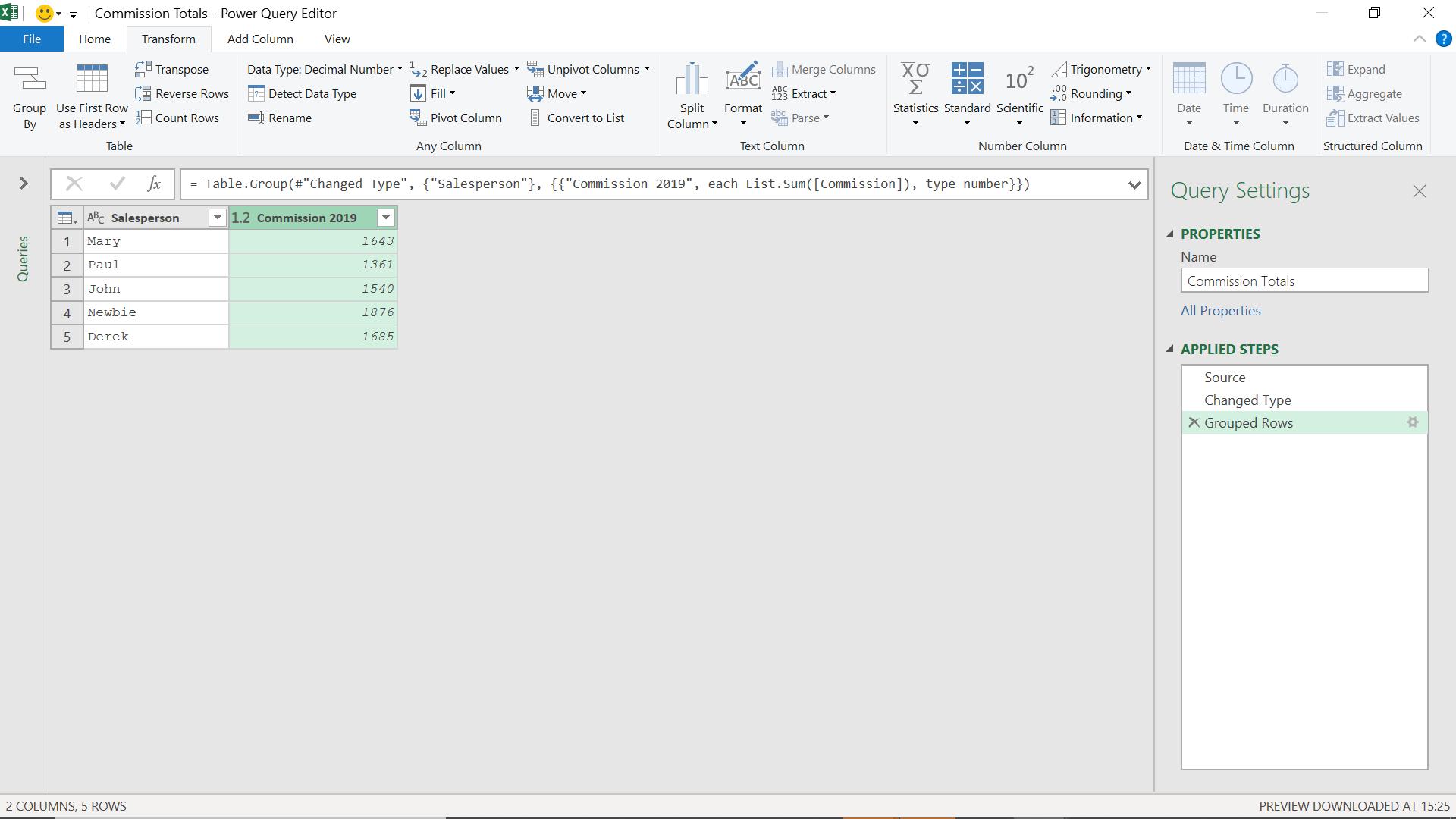
I need to find the total commission for each salesperson, so I use the grouping functionality on the ‘Transform’ tab. I group by Salesperson and sum the Commission.

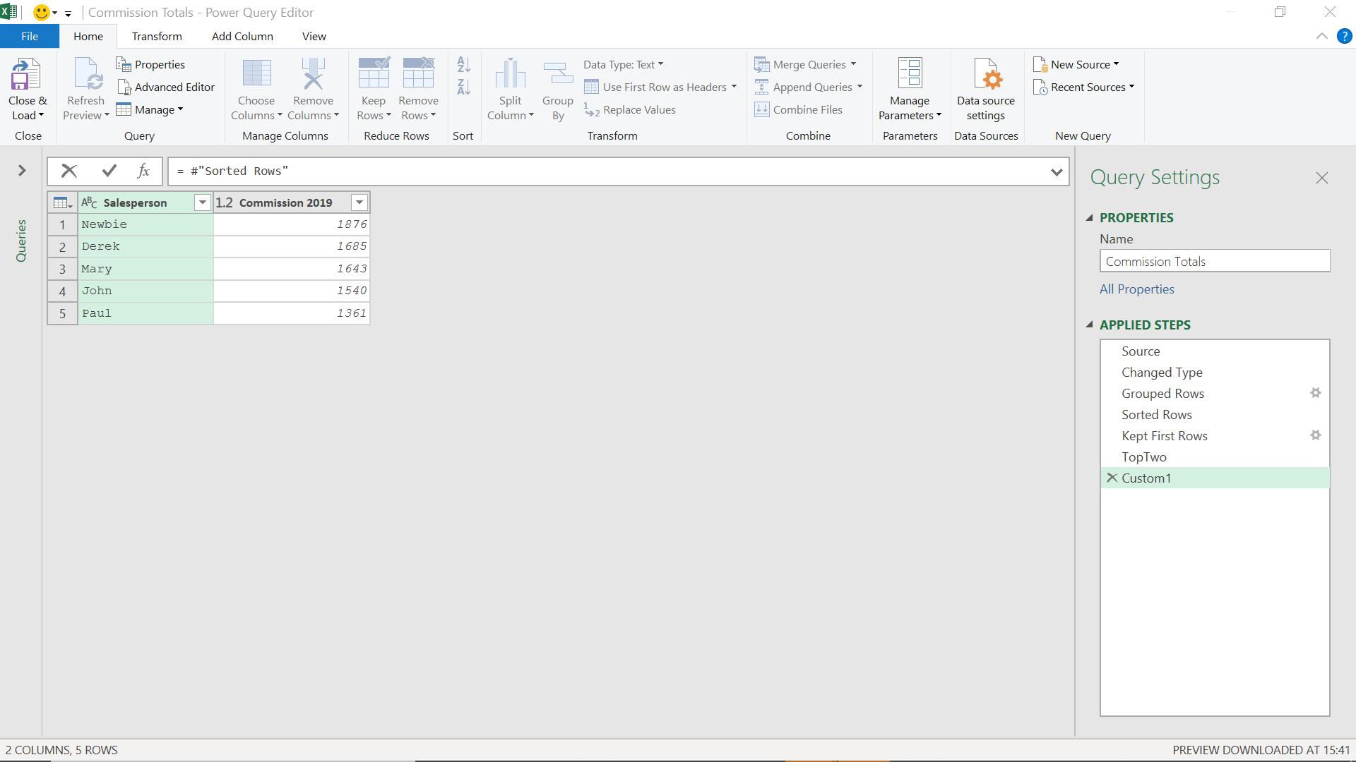
I can now apply a descending sort on Commission to get my top two salespeople.

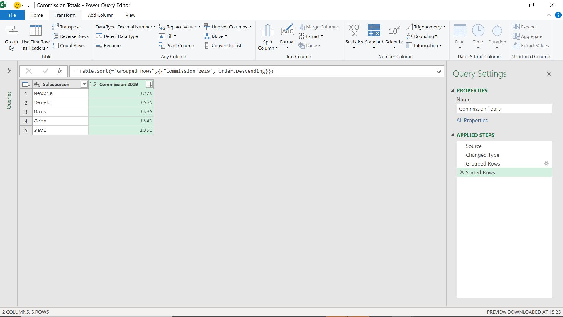
To get my top two salespeople, I can just take the top two rows.

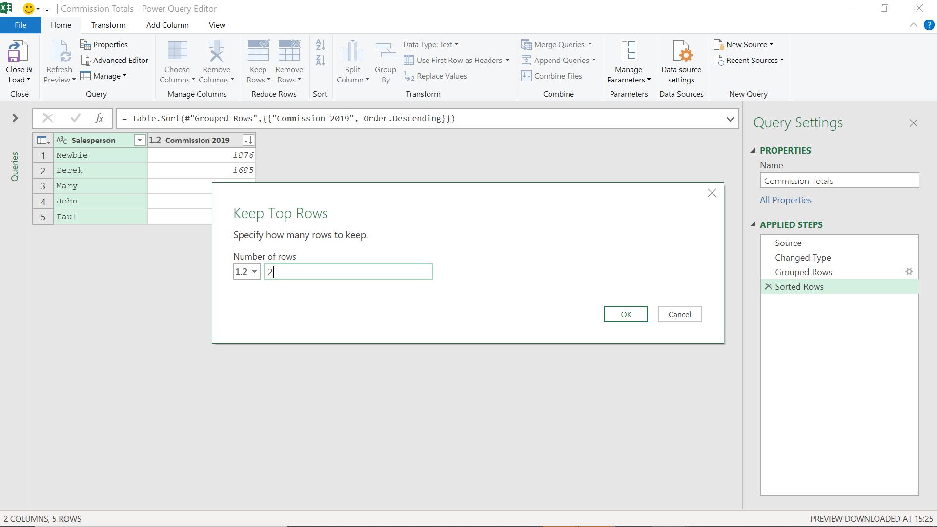
I choose to use the ‘Keep Rows’ functionality on the Home tab. This is more flexible than removing the bottom rows, as I don’t have to specify how many rows to remove.

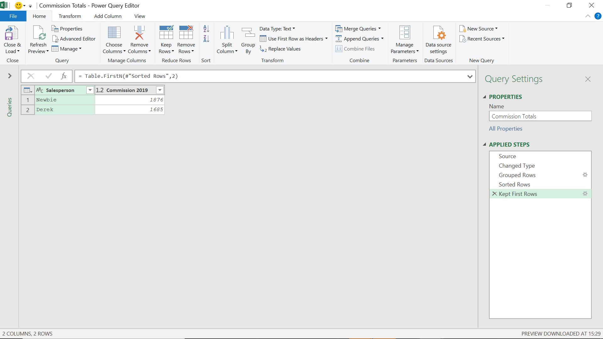
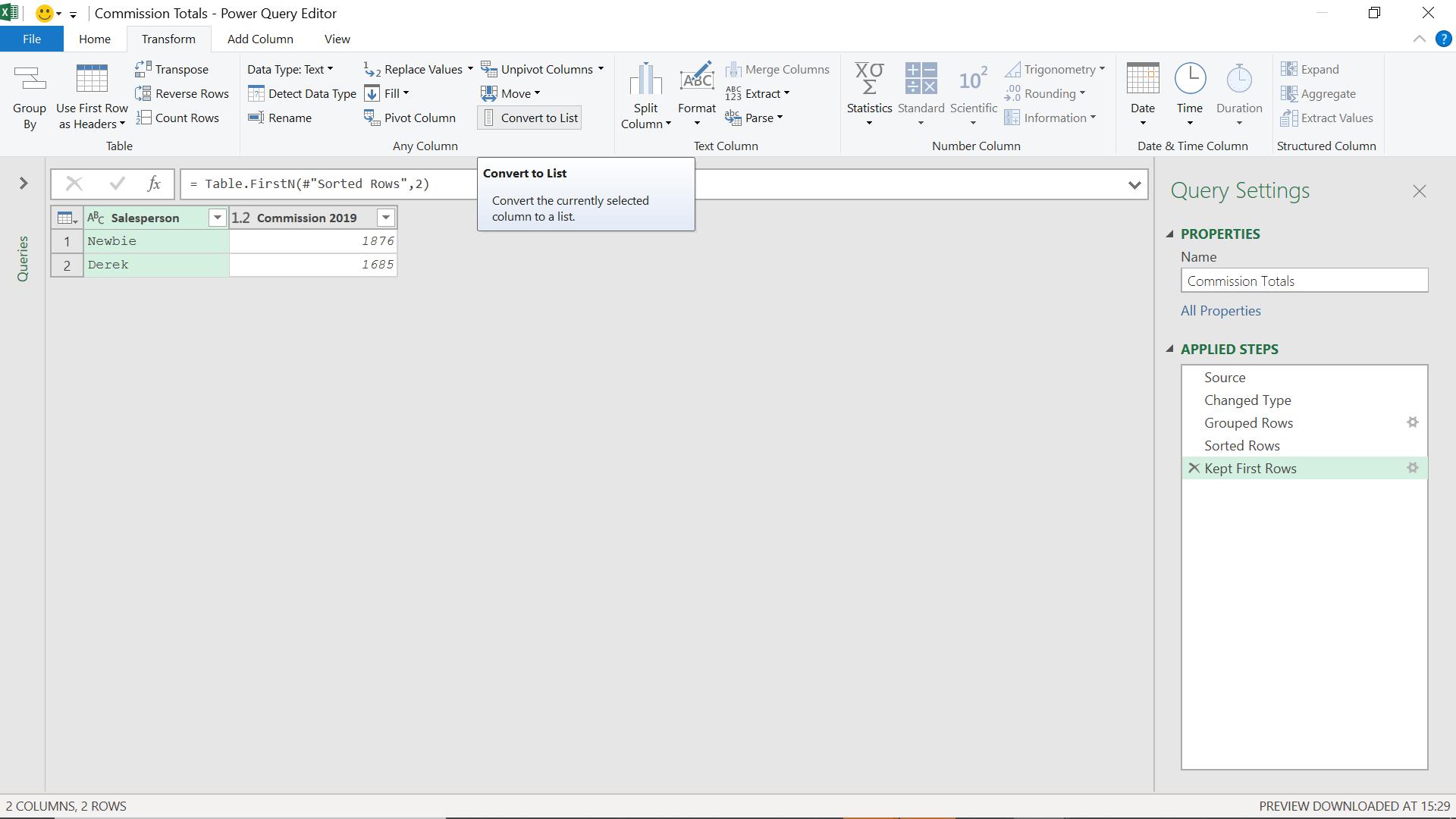
I now have my top two, and I am going to convert my salespeople column to a list by using the ‘Convert to List’ functionality on the Transform tab. I will use this later to reassemble my data.

I create my list:

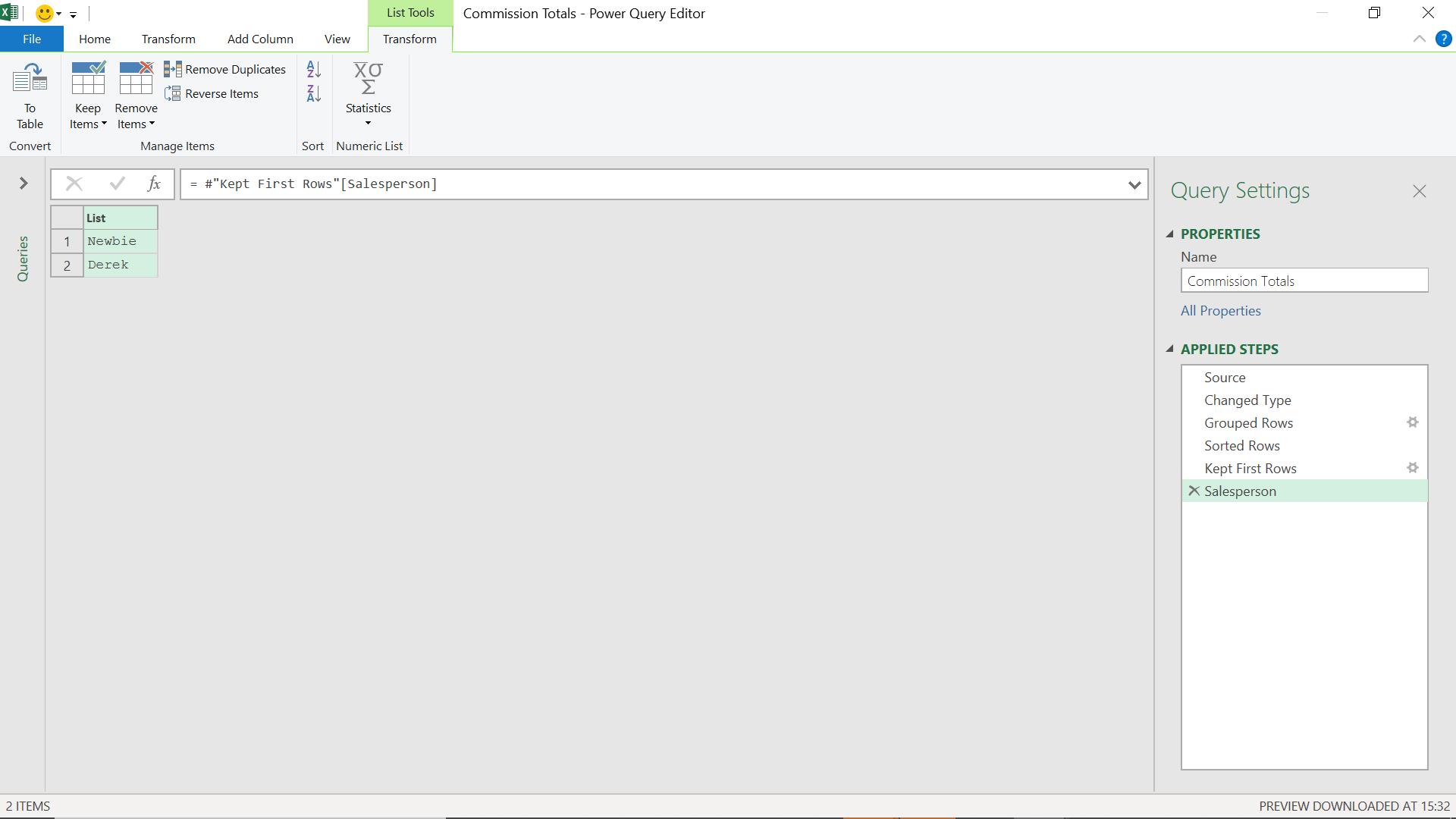
I rename the step to create my list TopTwo. Now, I need to deal with the others. I create a new step which refers to the data before I removed the bottom columns.

The M code I have used is:

which accesses the data before I removed the bottom rows.  This time, I need to remove the top rows using the remove rows functionality on the Home tab.

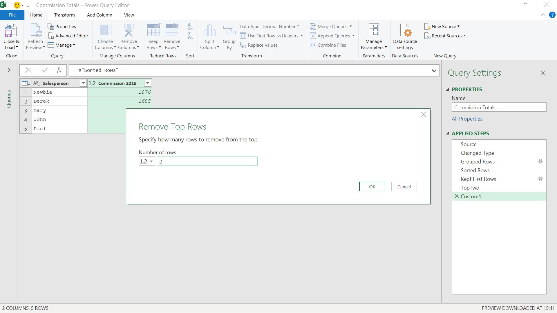
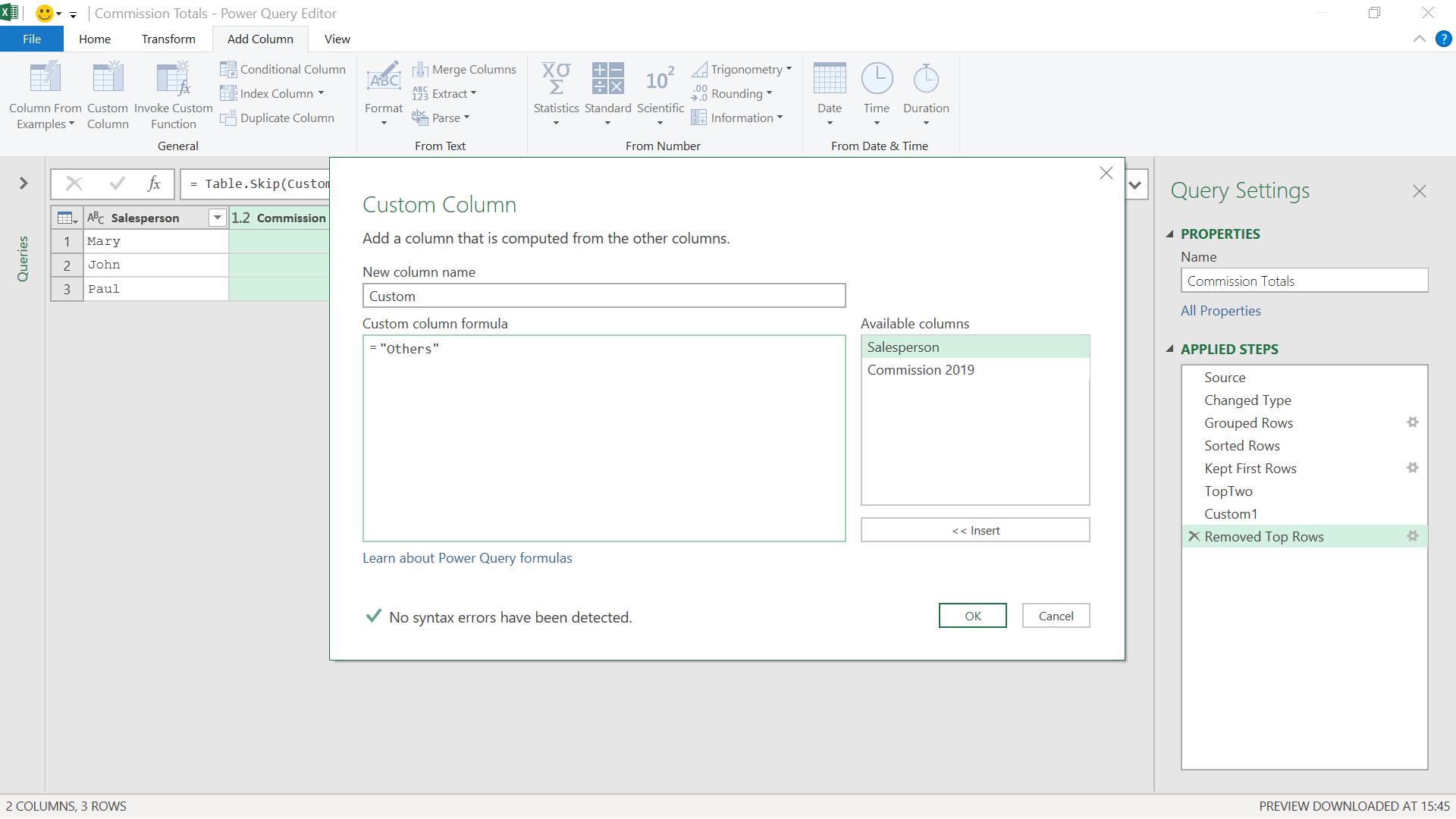
I remove the top two rows. To get the average to appear in each column, I will use grouping, but I need to group using a constant so that I can sum the commissions. To do this, I add a custom column from the ‘Add Column’ tab, which always has the same value. The value I am going to use is “Others”, viz.

I can now group my data from the Transform tab.

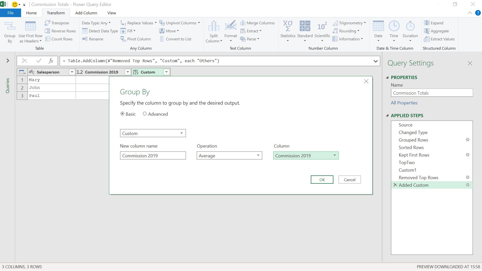
I group by Custom and create a new Commission 2019 column (yes, I know we are in 2020!) which will contain the average.

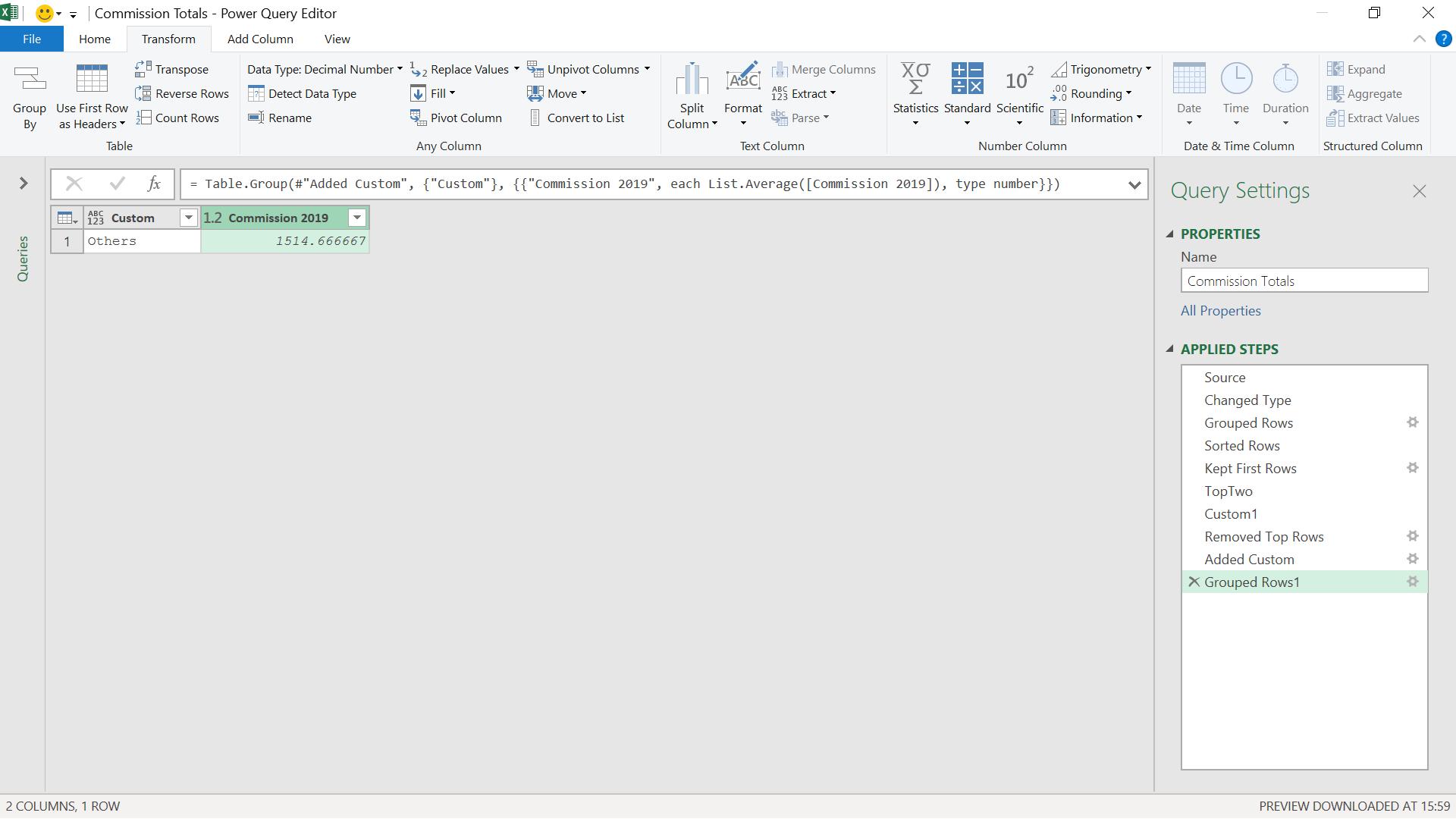
I have my data for the others, so I rename the step to Others and rename Custom to Salesperson. I am now ready to reassemble my data.

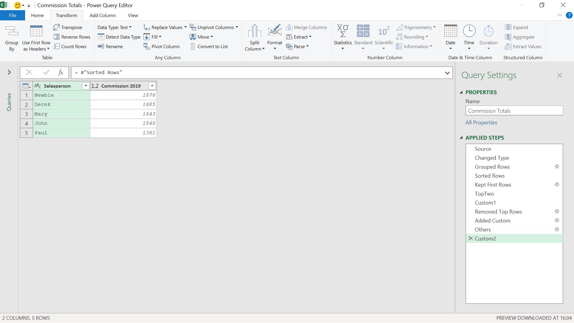
As I did earlier, I create a step to get back to my full data before I removed any rows. This will allow me to keep any columns that do not directly pertain to the calculation, and makes the method more flexible.

I need to select those rows which are associated with my top two.

 The M code I have used is:

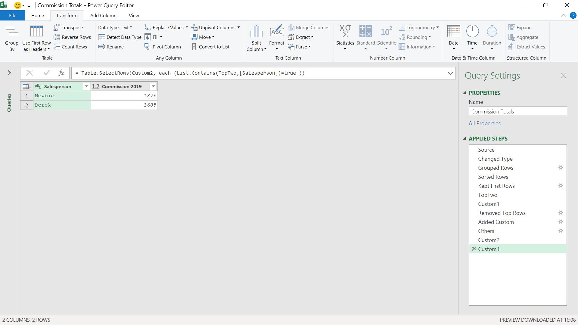
This gives me the data for my top two.  Now I need to add my ‘others’.  I do this by merging my table to itself, and then changing the M code generated.

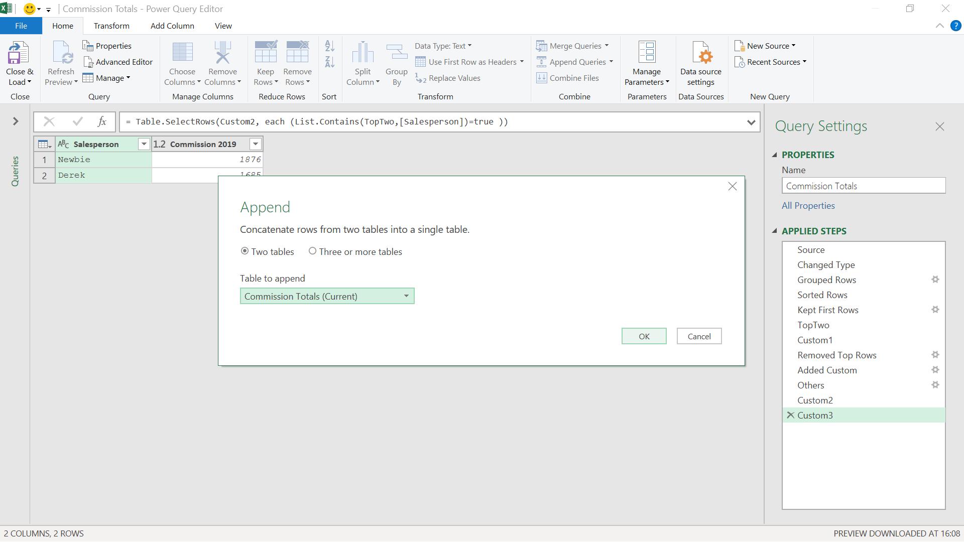
I check the M code generated.

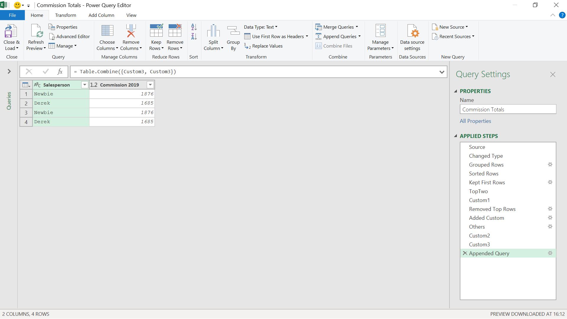
I have the M code

I change this to

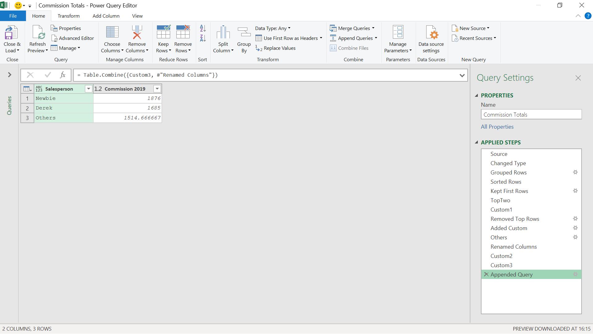
I now have my data in the form I wanted, with my top two salespeople and the others combined into one average commission.

Come back next time for more ways to use Power Query!