Power Query: Riveting Results Part 6

Welcome to our Power Query blog. This week, I complete the creation of the parameters from Excel cells.

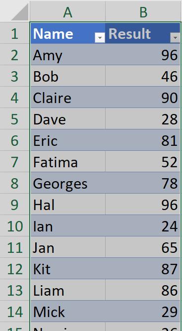
My salespeople are furloughed. This week, I continue looking at the exam results I created in Power Query: Riveting Results Part 1:

I will be grading the results and I will be using this example to explore parameters. Last week, I created a query from an Excel cell, which I will use as a parameter.

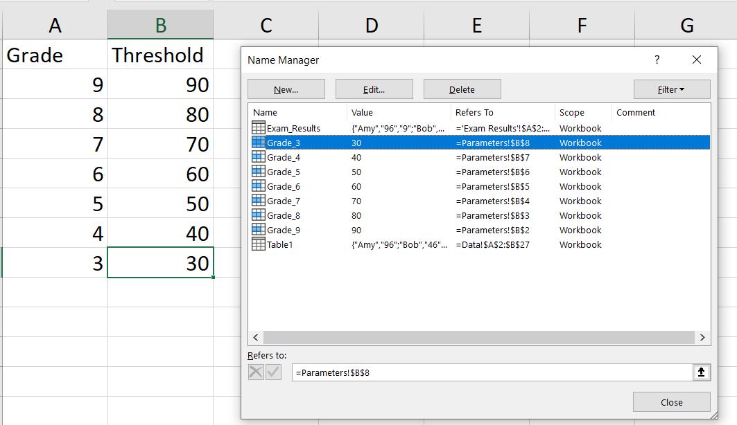
I now define names for all the cells that I want to use as parameters:

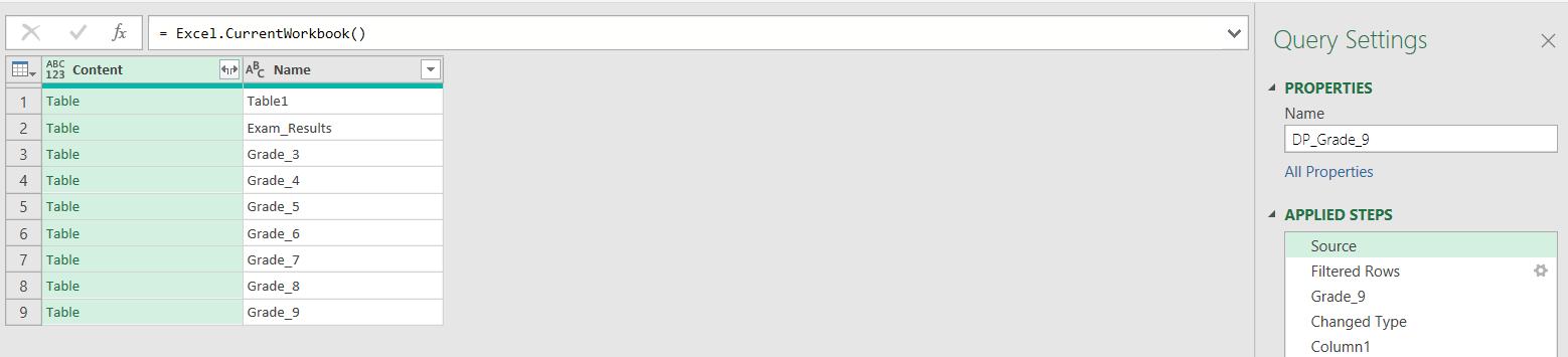
If I go to the DP_Grade_9 query in the Power Query Editor, I can view the Source step:

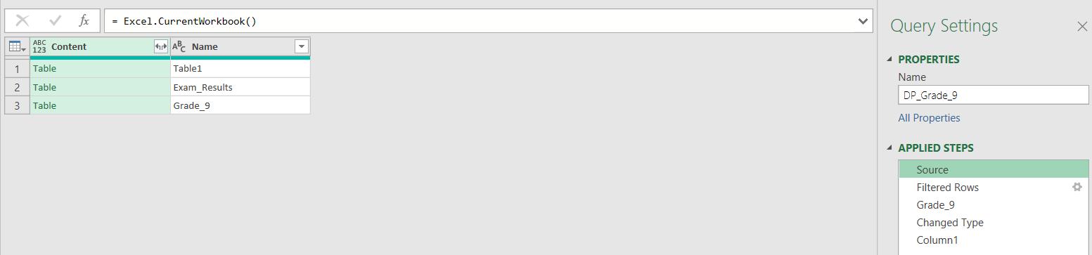
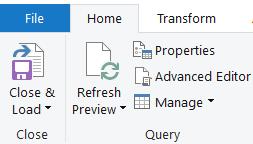
I ‘Refresh Preview’, using the option on the Home tab:

I notice that the other named cells now appear:

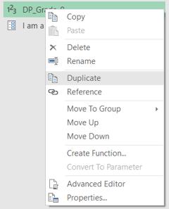
I can create a duplicate of DP_Grade_9:

I can use this as a template to create the other queries:

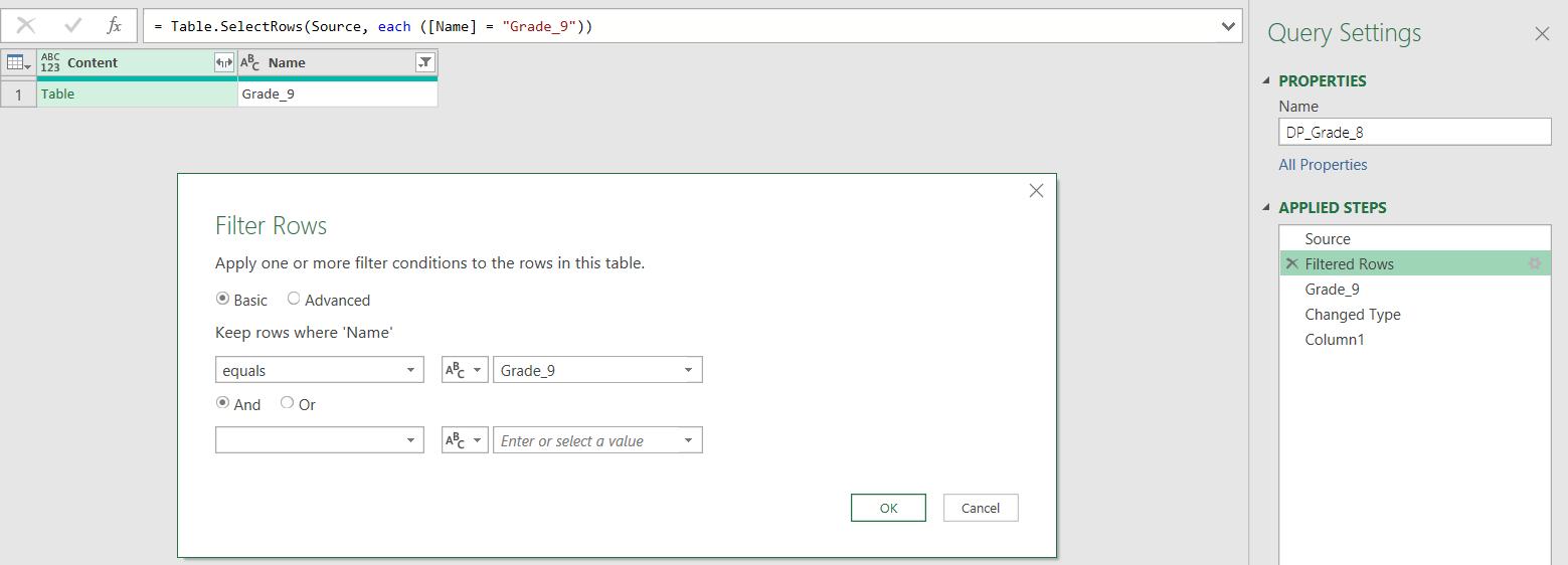
I have renamed the duplicate query, and I click on the cog next to ‘Filtered Rows’ to amend the value of Name selected to ‘Grade_8’. Note that the step ‘Grade_9’ will also need to be edited, as I will see as soon as I click OK and move to that step.

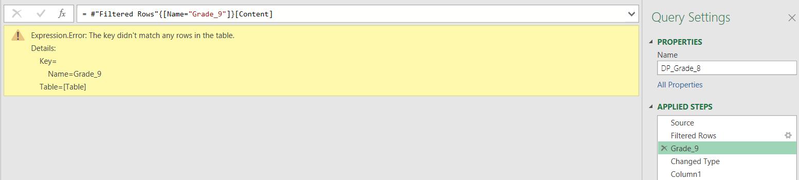
This step is trying to expand the Content column which corresponds to the Name ‘Grade_9’.  The M code is:

I can change this to:

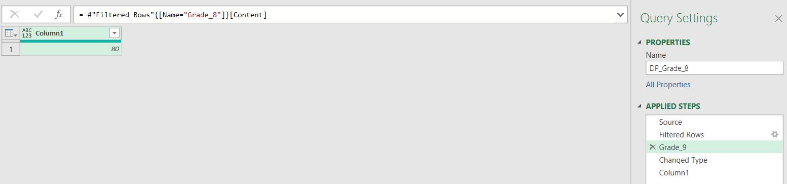
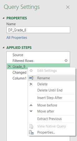
I have the correct result, but I should also right-click on the step and change the name to avoid confusion:

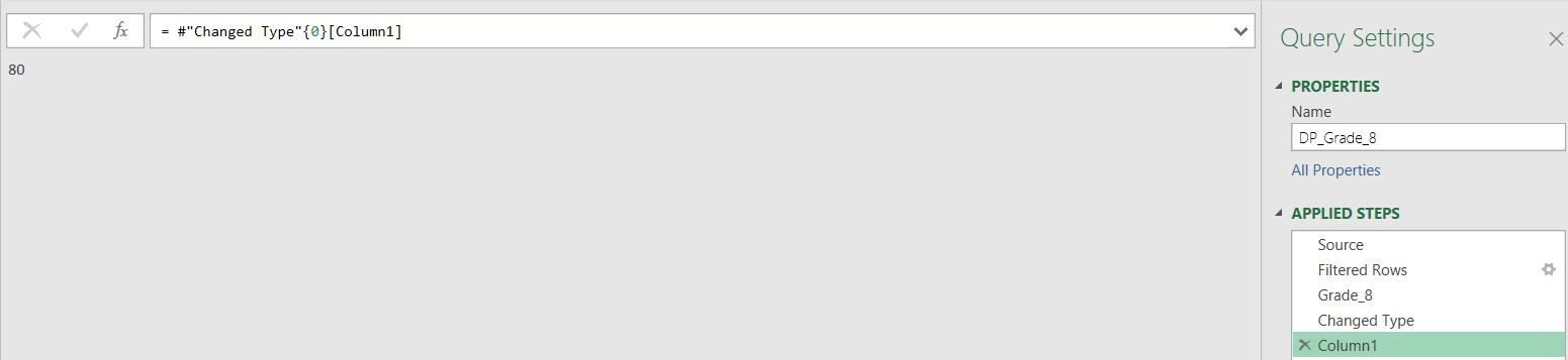
I have completed this query:

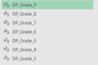
I repeat this process for the other named cells:

Next time, I will apply these parameters to the Exam Results query and check that any changes to the Excel cells affect the outcome of the query.

Come back next time for more ways to use Power Query!