
Power Query: Riveting Results Part 4
5 January 2022
Welcome to our Power Query blog. This week, I start to create a parameter from a cell in Excel.
My salespeople are taking a really long break. This week, I continue looking at the exam results I created in Power Query: Riveting Results Part 1:
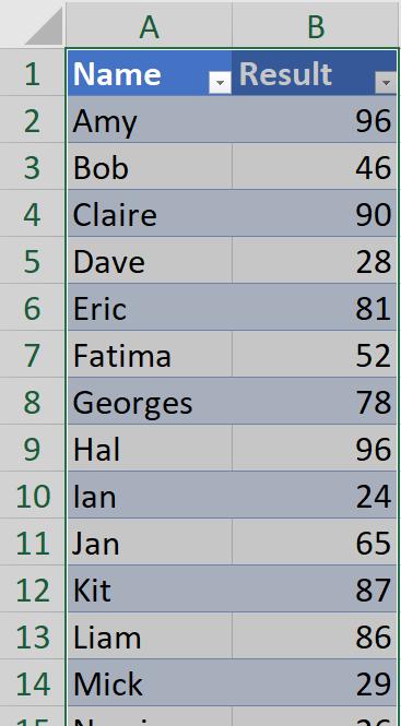
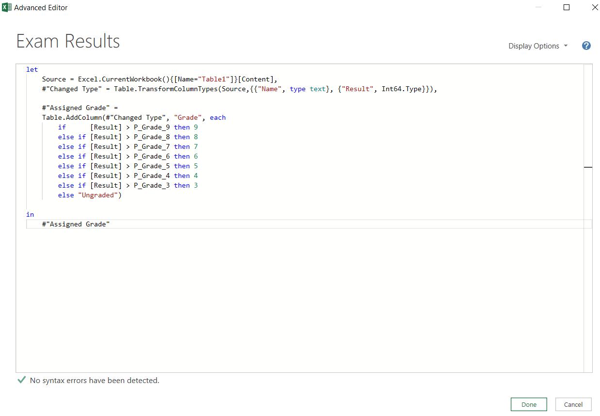
I will be grading the results, and I will be using this example to explore parameters. Last week, I added parameters to the query Exam Results.
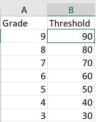
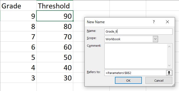
Whilst I can change these parameters in Power Query, I’d now like to have parameters that I can change from Excel. On a new Excel Sheet, I have some data for the thresholds:
I start by defining a Name for the first threshold. I can do this by selecting the cell and right-clicking:
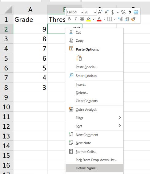
I define the Name to be ‘Grade_9’:
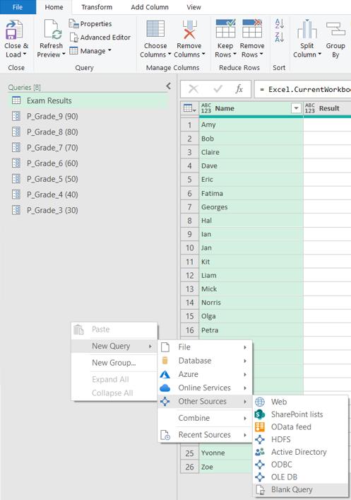
I can now see this in Power Query. In the Power Query Editor, I create a new Blank Query. I can do this by right-clicking in the Queries pane (this is one of several methods to create a Blank Query):
In my Blank Query, I enter the following M code:
= Excel.CurrentWorkbook()
This will show me what is in the current Excel Workbook:
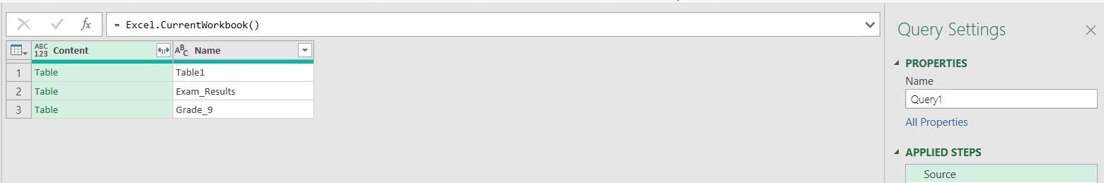
There is the Grade_9 I created. The value will be in the ‘Table’ next to it.
Next time, I will extract this data into a parameter, and look at why this is different from a parameter created from the ‘Manage Parameters’ dialog.
Come back next time for more ways to use Power Query!