Power Pivot Principles: Introducing the VALUES Function

Welcome back to the Power Pivot Principles blog.  This week, we will talk about the VALUES function in DAX.

The VALUES function, similar to the DISTINCT function, returns a one-column table that contains the distinct values from a specified column.  Duplicate values are removed and only unique values are returned.  This function cannot be used to return values into a cell or column on a worksheet, nut rather it is nested within a formula, to get a list of distinct values that may be counted or used to filter / sum other values (say).

The VALUES function has the following syntax:

Let’s consider an example.  Yet again, here is sales data from 2016 to 2019 for a number of stores, where they track sales by ‘Product Key’ and ‘Customer Key’:

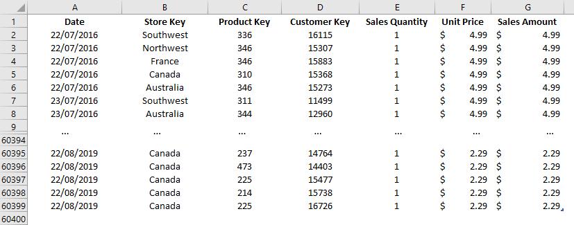
We want to know the number of unique customers each store gains over time.

To do this, first, we will load the data to the Power Pivot Data Model, by highlighting the whole data, going to the ‘Power Pivot’ tab on the Ribbon and clicking ‘Add to Data Model’.  We then rename the tables as Sales.  We also add a Calendar Table, which will later be used in our PivotTable, and name it Calendar.  We will also define the relationships between Sales and Calendar by switching to ‘Diagram View’ in the Home tab and dragging the Date field to connect the two tables.

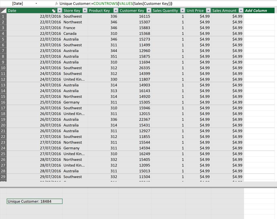
To count the number of unique customers, we will create a measure ‘Unique Customer’ and use the VALUES function:

In here, we may not bring the list of values that VALUES returns directly into a column.  There would be a thousand of them, while we only want to know the total!  Therefore, we need to nest the VALUES function in the COUNTROWS function.  The measure returns a result of 18,484 unique customers, which makes sense, but is not the end result that we want…

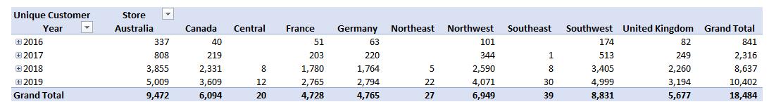
Going back to Excel, we create a PivotTable in a new worksheet. Here we drag Year from the ‘Calendar’ table into Rows field, ‘Store Key’ into the Columns field, and ‘Unique Customer’ into the Values field. Thus, we have a PivotTable showing the number of unique customers by stores and by years:

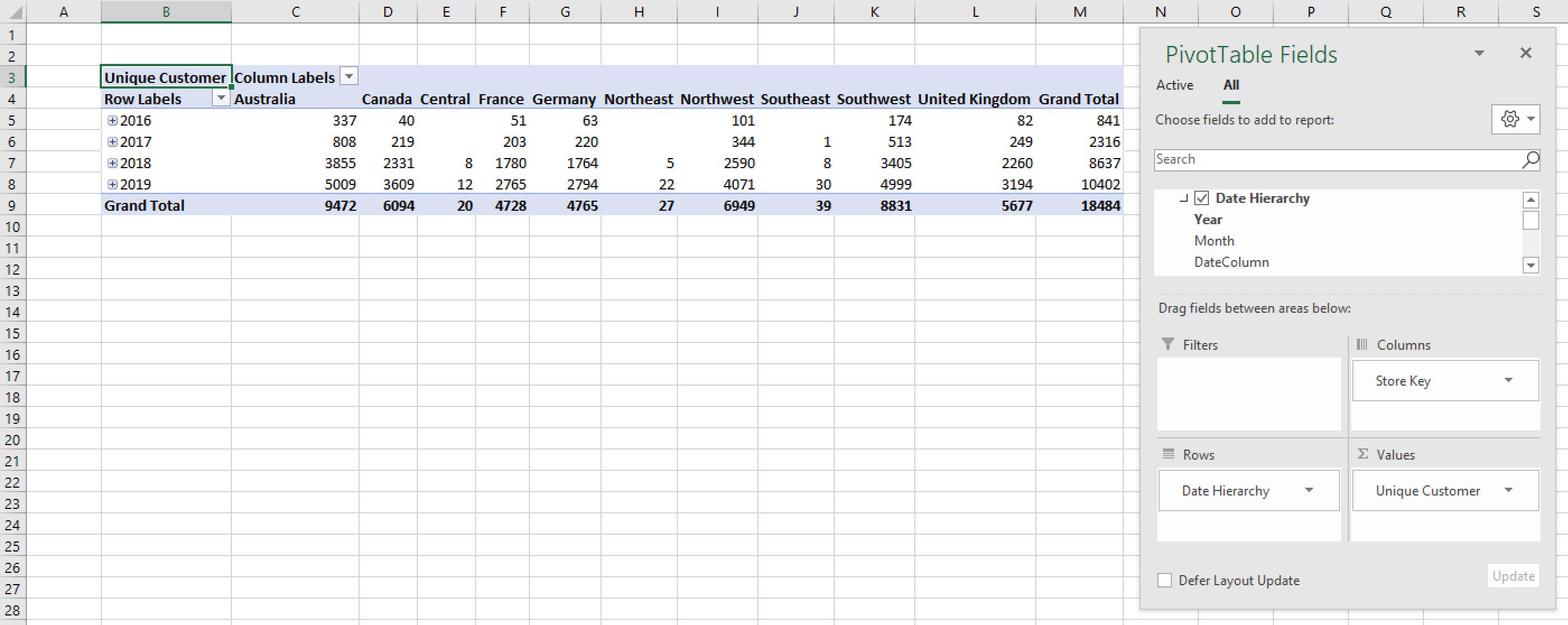
Just to double check, the Grand Total of Grand Totals is 18,484 customers, which coincides with the number generated from our Data Model’s measure!

That’s it for this week!


Stay tuned for our next post on Power Pivot in the Blog section. In the meantime, please remember we have training in Power Pivot which you can find out more about >here. If you wish to catch up on past articles in the meantime, you can find all of our Past Power Pivot blogs here.