
Power Pivot Principles: Selecting from Multiple Lookup Values
12 November 2019
Welcome back to the Power Pivot Principles blog. This week, we are going to introduce a method to extract a single value from the group text columns.
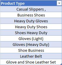
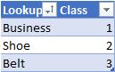
In our previous blog, we introduced a method to group text columns into new categories. For example, consider the situation below. We have data tables containing Product Type and the Lookup categories. We can create a column that will highlight if any one of the values from the Lookup table is present in the Product Type column. For instance, if the Product Type value is ‘Leather Belt’, we would want the column to recognise that that value had ‘Belt’ in it.
However, in some cases, multiple values would be captured by the formula and it is hard to decide which category should be given to a specific type. For example, if the product type is ‘Business Shoes’, the result would return ‘BusinessShoe’, as shown below:
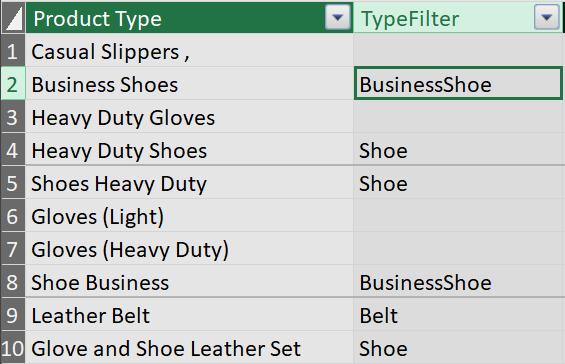
Both categories Business and Shoe are listed in the lookup table, and the formula returns both values in the context. However, only one category should be applied to the Product Type: the value should be either Business or Shoe in this case. Therefore, we need to find a method to split the content if there are multiple categories.
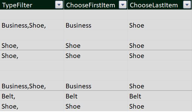
After loading the Product Type table and Lookup table into Power Pivot, we create a calculated column TypeFilter with the formula below:
=CONCATENATEX(
'Lookup Table',
IF(
SEARCH(FIRSTNONBLANK('Lookup Table'[Lookup],1),'Product Type'[Product Type],,999) <> 999,
'Lookup Table'[Lookup]&",",
""
)
)
This code is very similar to the code we used in our previous blog, with one key difference. Instead of returning with the 'Lookup Table'[Lookup], we change it to 'Lookup Table'[Lookup]&”,”. By adding the delimiter of a comma, we can split the content by using other text functions such as MID, LEFT and RIGHT etc.
If we take the first selection criteria as the main category, we may create a calculated column ChooseFirstItem and use the LEFT function to determine the context of first category, as shown below:
=LEFT(
'Product Type'[TypeFilter],
SEARCH(",",'Product Type'[TypeFilter],,999)-1
)
The result would be:
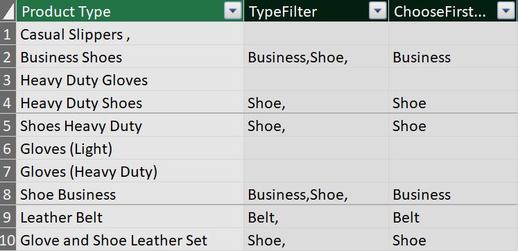
The SEARCH function returns the location of the comma delimiter and the LEFT function extracts the number of characters, as determined by the SEARCH function. If the second category should be considered as the main category, we need a few extra steps to extract the second context as required.
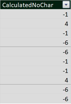
We can create a calculated column CalculatedNoChar to search the location of second delimiter, with the start position at the first delimiter, as shown below:
=SEARCH(",",
'Product Type'[TypeFilter],
SEARCH(",",
'Product Type'[TypeFilter],,0)+1,0
)
-SEARCH(",",
'Product Type'[TypeFilter],,0
)-1
The result would be:
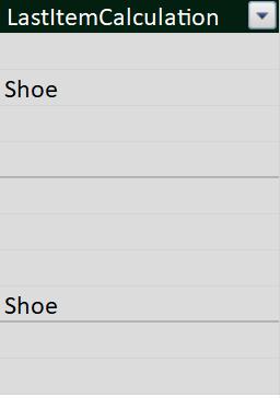
Next, we can create a calculated column LastItemCalculation and use the MID function to find the second category, with the condition that the value of CalculatedNoChar must be greater than zero.
=IF('Product Type'[CalculatedNoChar]>0,
MID('Product Type'[TypeFilter],
SEARCH(",",'Product Type'[TypeFilter],,0)+1,
'Product Type'[CalculatedNoChar]),BLANK()
)
The result would be:
The last step is to create a calculated column ChooseLastItem . We can use the IF function to return the second category if the value in LastItemCalculation is not blank, as shown below:
=IF(ISBLANK('Product Type'[LastItemCalculation]),
'Product Type'[ChooseFirstItem],
'Product Type'[LastItemCalculation]
)
The result would be:
That’s it for this week!
Stay tuned for our next post on Power Pivot in the Blog section. In the meantime, please remember we have training in Power Pivot which you can find out more about here. If you wish to catch up on past articles in the meantime, you can find all of our Past Power Pivot blogs here.