
Power Pivot Principles: Grouping Text Columns with New Categories Dynamically using an Input Table – Part 2
9 July 2019
Welcome back to our Power Pivot blog. Today, we show you how use set up slicers to dynamically segregate text data based on text inputs.
Last week we showed you how to group text columns with new categories dynamically using an input table. This week, let’s expand on that concept.
Imagine we have the following data table, noting that this screenshot is not exhaustive:
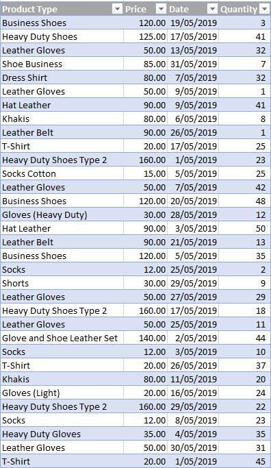
We would like to be able to group the Product IDs by a new category. These categories are detailed in the following table:
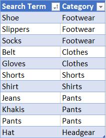
In summary, if the Product ID text contains ‘Shoe’ the new column will display ‘Footwear’, and if the text contains ‘Jeans’ the new column will return with ‘Pants’, etc.
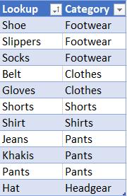
How do we do this? Well, from our last blog, we used the following single column lookup table:

This time we can alter our lookup table and have two columns, one column for the Lookup value and the other for the category name we wish to return:
After loading both tables into Power Pivot, we create a calculated column with the following code:
=CONCATENATEX(
'LookupTable',
IF(
SEARCH(
FIRSTNONBLANK( 'LookupTable'[Lookup],
1
),
'DataTable'[Product Type],
,
9999
)
<> 9999,
'LookupTable'[Category],
""
)
)
This code is very similar to the code we used last week, with one key difference. Instead of returning with the 'LookupTable'[Lookup], we change it to 'LookupTable'[Category]. This way, the column will be populated with the new category that we wish to assign to each row:
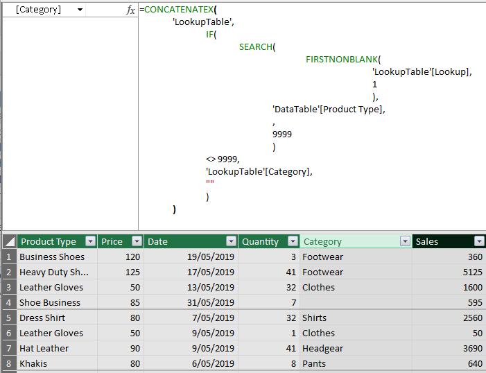
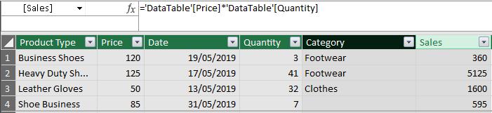
We will also have to create a Sales column that multiplies the Price by the Quantity:
='DataTable'[Price]*'DataTable'[Quantity]
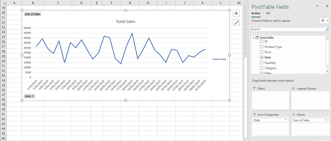
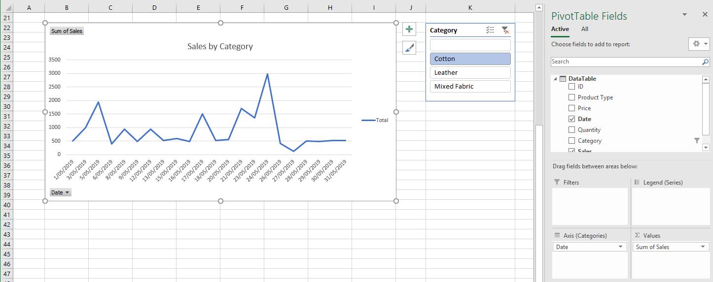
We can now create the following PivotChart:
The next step is to create a Slicer for our new Category column:
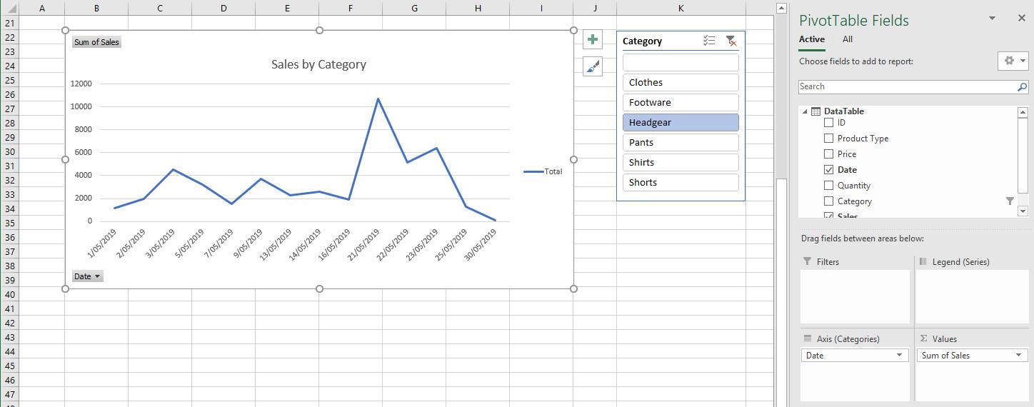
We can now filter our graph to display different categories of our data!
The best part is that if we wish to change the categories or lookup values all we have to do is change the values in our lookup table, refresh the links in Power Pivot and our chart will update accordingly.
For example, updating our lookup table to:
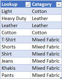
and refreshing the links in Power Pivot, our PivotChart will be updated as follows:
That’s it for this week, happy pivoting!
Stay tuned for our next post on Power Pivot in the Blog section. In the meantime, please remember we have training in Power Pivot which you can find out more about >here. If you wish to catch up on past articles in the meantime, you can find all of our Past Power Pivot blogs here.