
Power Pivot Principles: Irregular Month-End Reporting Case – Part 3
1 September 2020
Welcome back to the Power Pivot Principles blog. This week, we continue with our irregular month-end reporting case study.
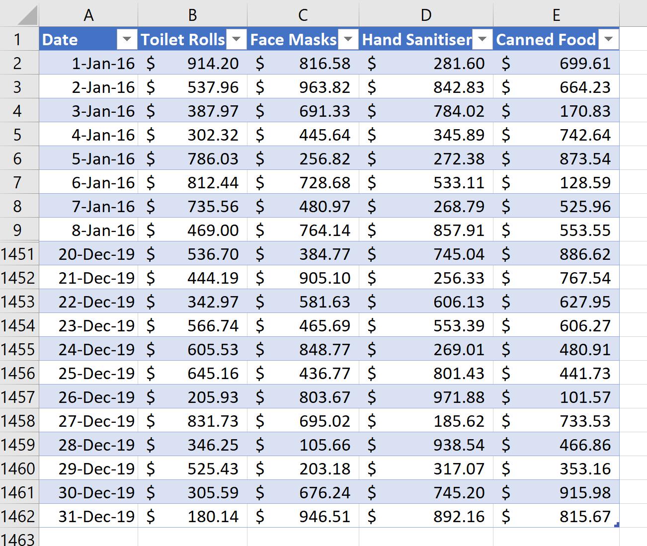
To recap, we have a sales data set of four product lines in a supermarket over four years. This supermarket has a rule for month-end reporting, which is the reporting end of month day is the final Thursday of a month, regardless of whether it matches the end of the calendar month.
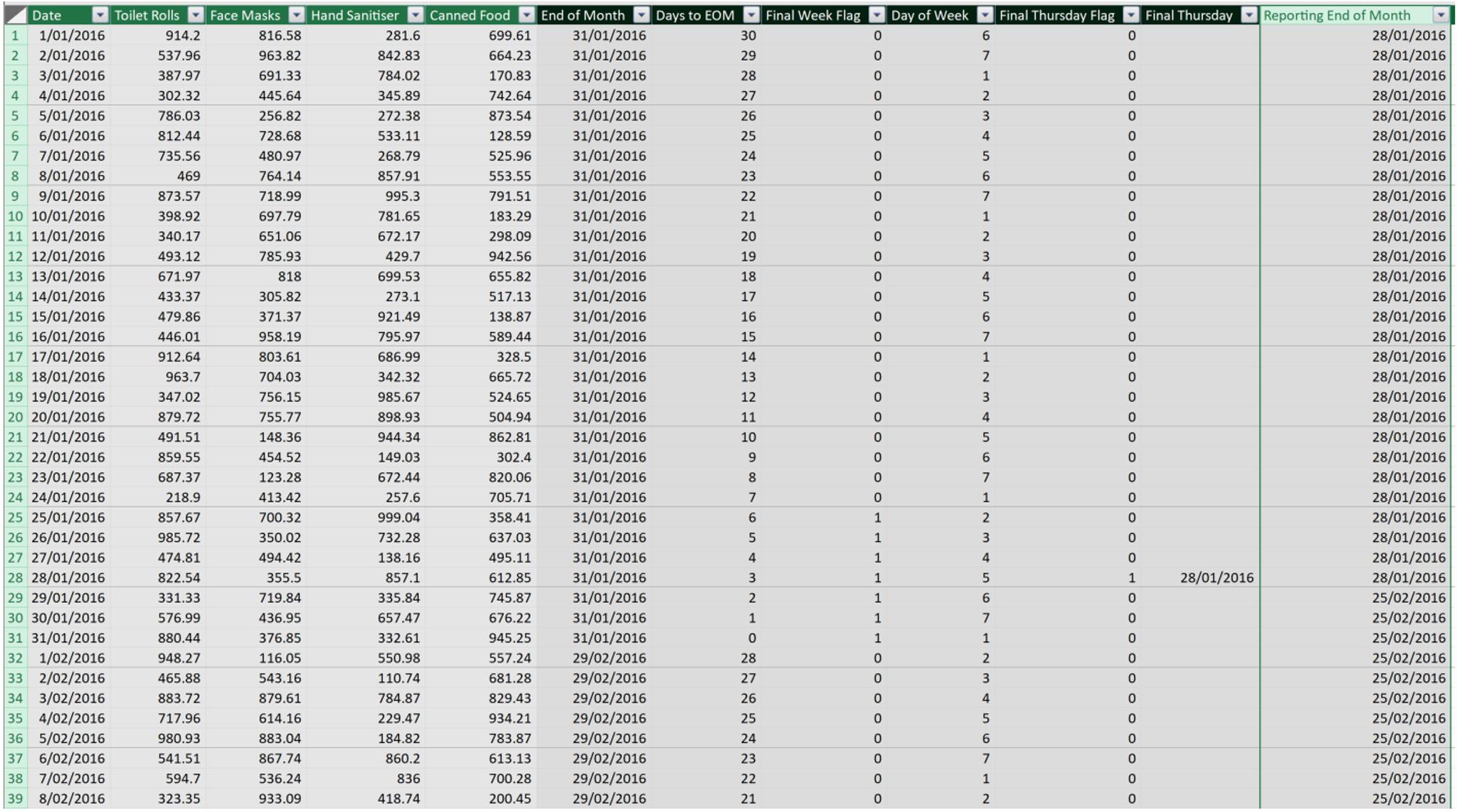
By using the EOMONTH and the WEEKDAY functions to compare the logic or by using ‘Fill Up’ calculations, we worked out the final Thursday of each month to be the ‘Reporting End of Month’:
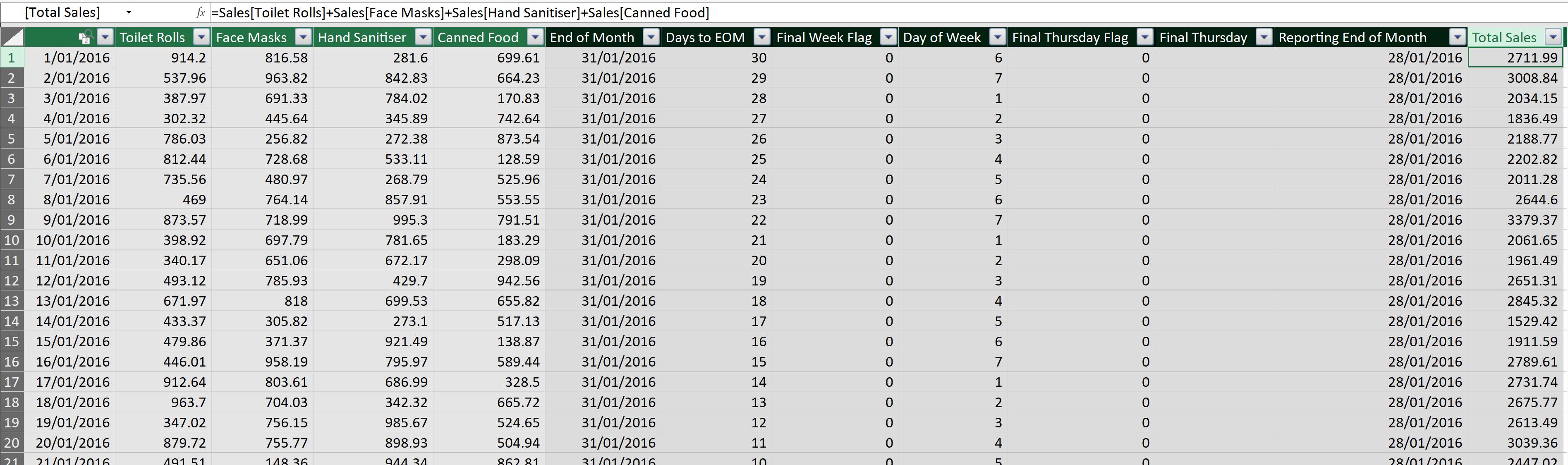
Now, we want to get some insights about the sales of each month. First, in the Sales table, we create a calculated column ‘Total Sales’:
=Sales[Toilet Rolls] + Sales[Face Masks] + Sales[Hand Sanitiser] + Sales[Canned Food]
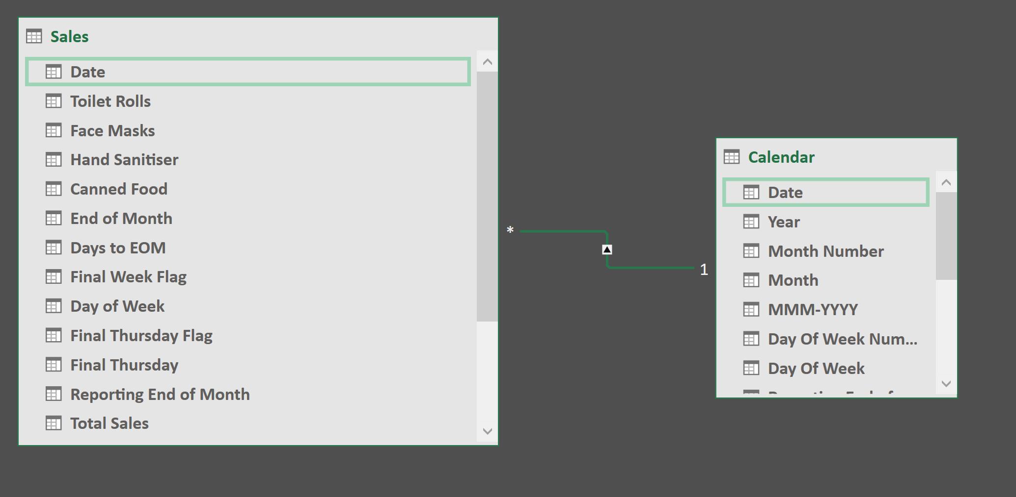
Then, we create a Calendar Table, by going to the Design tab on the Ribbon of the Power Pivot window, choose Date Table à New. After the Calendar Table is created, we navigate to the Diagram view to form a relationship between the two tables, by connecting the Dates columns:
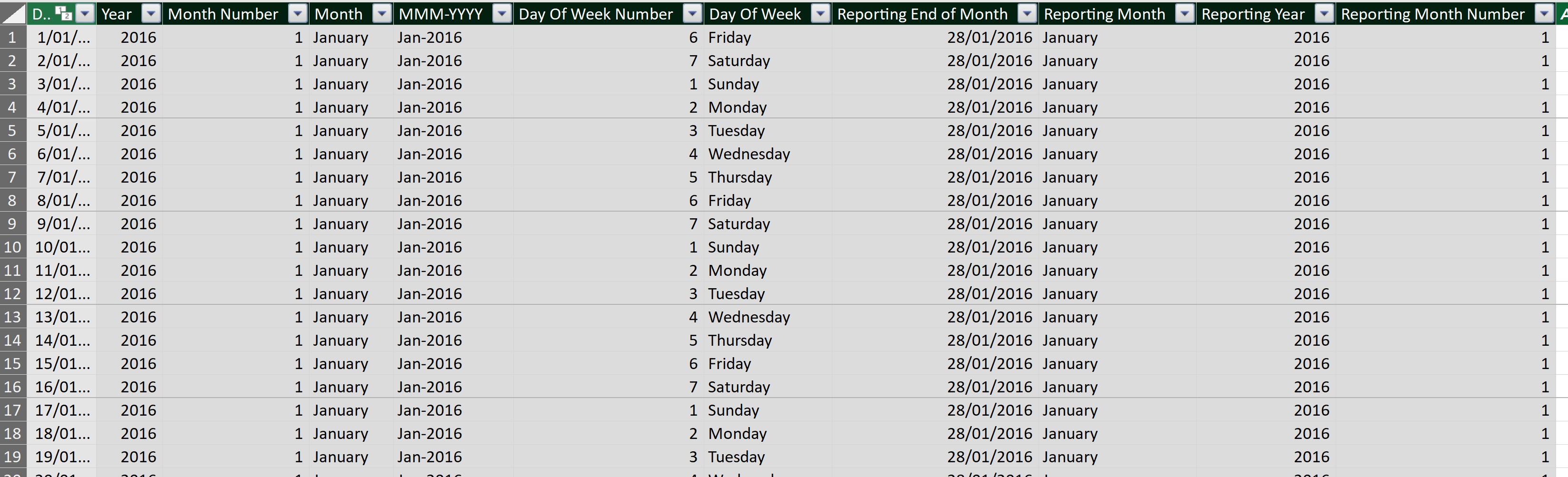
Since we have an irregular reporting rule, in the Calendar Table, we will create four more columns to specify this rule. We will use the LOOKUPVALUE function to get the ‘Reporting End of Month’ in the Calendar Table, and then get the related ‘Reporting Month’, ‘Reporting Year’, ‘Reporting Month Number’ which we will use later in our PivotTable:
Reporting End of Month = LOOKUPVALUE(Sales[Reporting End of Month],Sales[Date],'Calendar'[Date])
Reporting Month = FORMAT([Reporting End of Month],"MMMM")
Reporting Year = YEAR([Reporting End of Month])
Reporting Month Number = MONTH([Reporting End of Month])
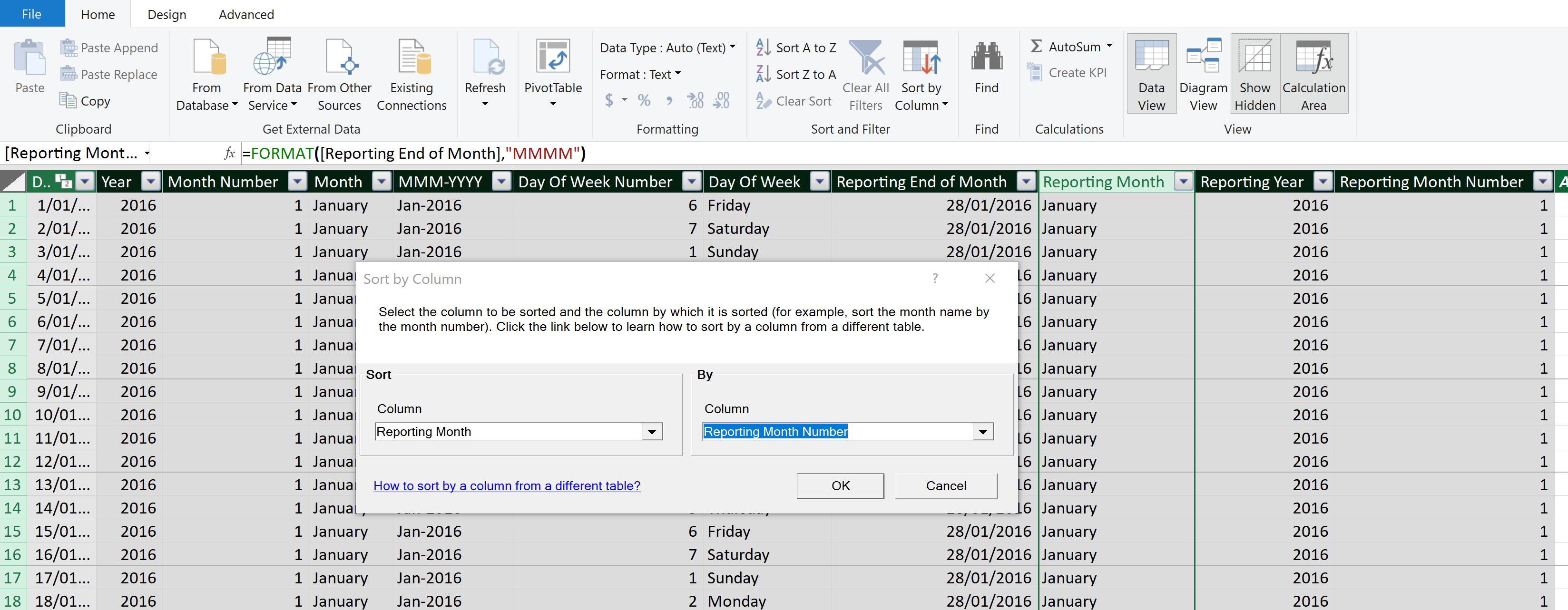
Next, we need to sort the ‘Reporting Month’ by the ‘Reporting Month Number’, otherwise, it will be sorted alphabetically in our PivotTable i.e. April goes first instead of January. We highlight the ‘Reporting Month’ column, go to Home -> Sort by Column -> Sort by Column… and choose ‘Reporting Month Number’ in the ‘By Column’ box:
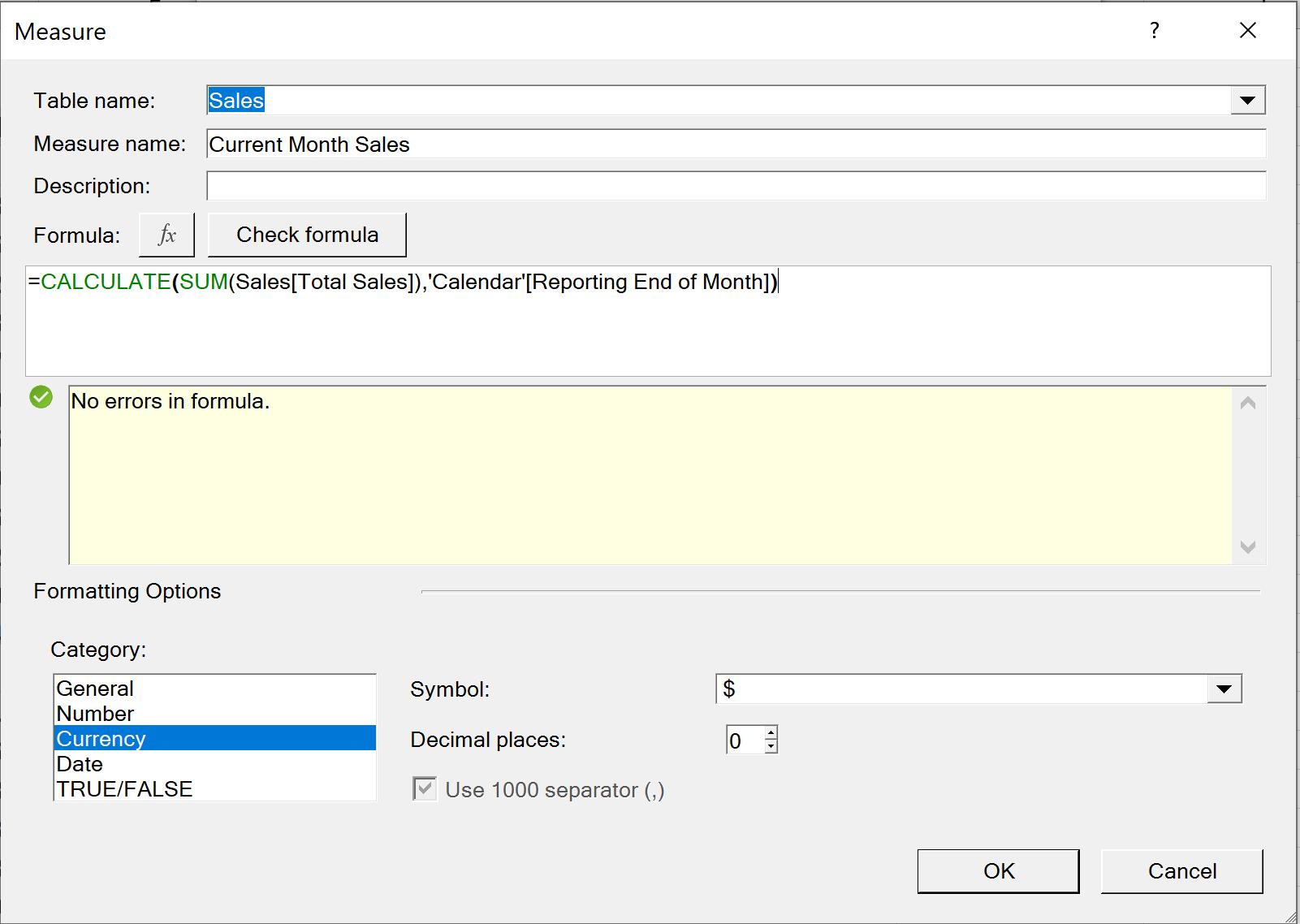
We are now prepared! Now, we will create another measure ‘Current Month Sales’:
=CALCULATE(SUM(Sales[Total Sales]), 'Calendar'[Reporting End of Month])
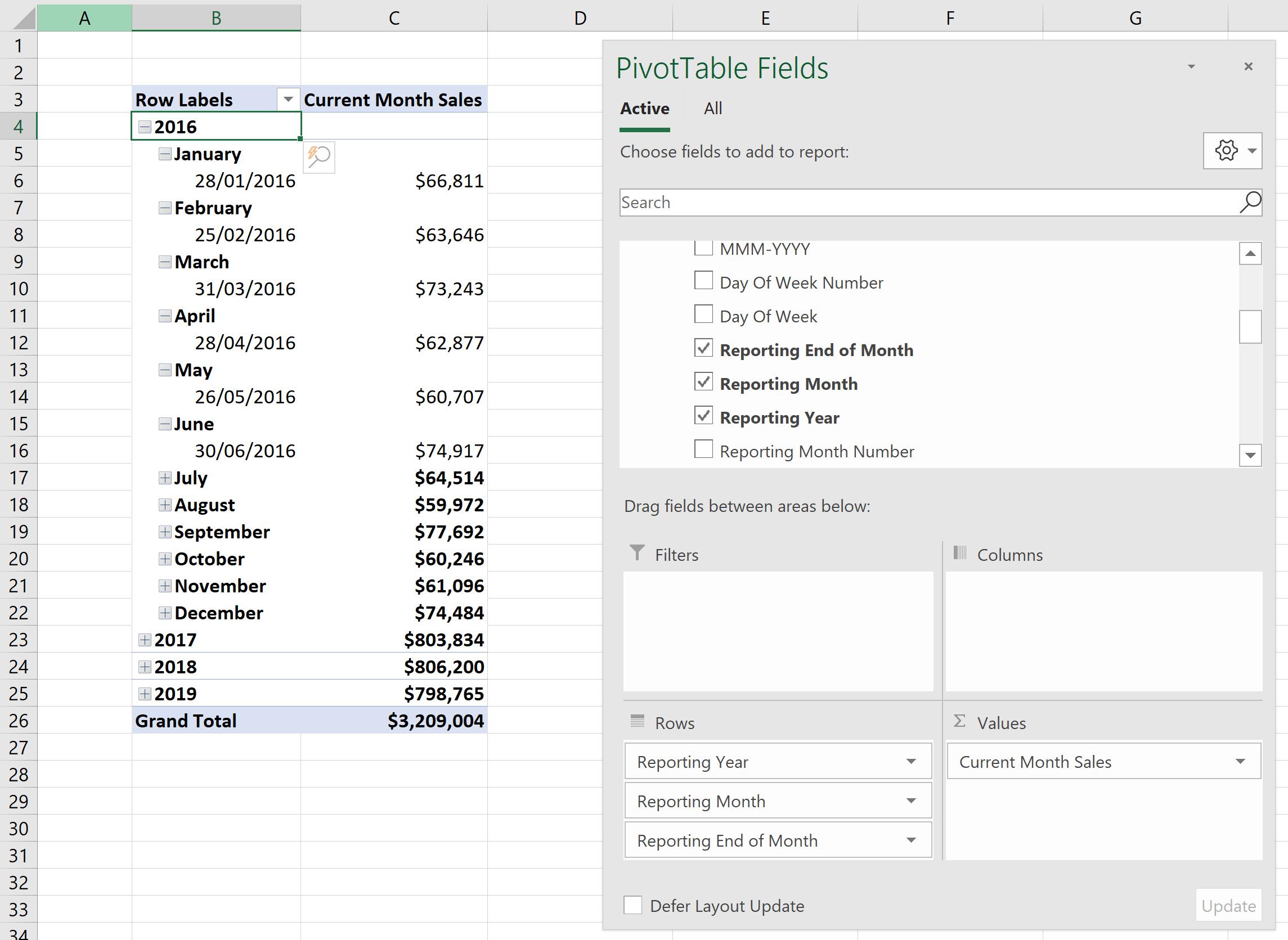
We will create a PivotTable by dragging the ‘Reporting Year’, ‘Reporting Month’, ‘Reporting End of Month’ fields (from the Calendar Table -> More Fields) to Rows and ‘Current Month Sales’ (from the Sales table) to Values. We can see the sales by month ending on the final Thursday of the month, viz.
That’s it for this week!
Stay tuned for our next post on Power Pivot in the Blog section. In the meantime, please remember we have training in Power Pivot which you can find out more about here. If you wish to catch up on past articles in the meantime, you can find all of our Past Power Pivot blogs here.