Power Pivot Principles: Power Pivot Principle: Introducing the RELATEDTABLE function

Welcome back to the Power Pivot Principles blog.  This week, we consider the RELATEDTABLE function in DAX.

The RELATEDTABLE function evaluates a table expression in a context, modified by the given filters and returns a table of values.  This function is a shortcut for the CALCULATETABLE function, but with no logical expression.  It follows the syntax:

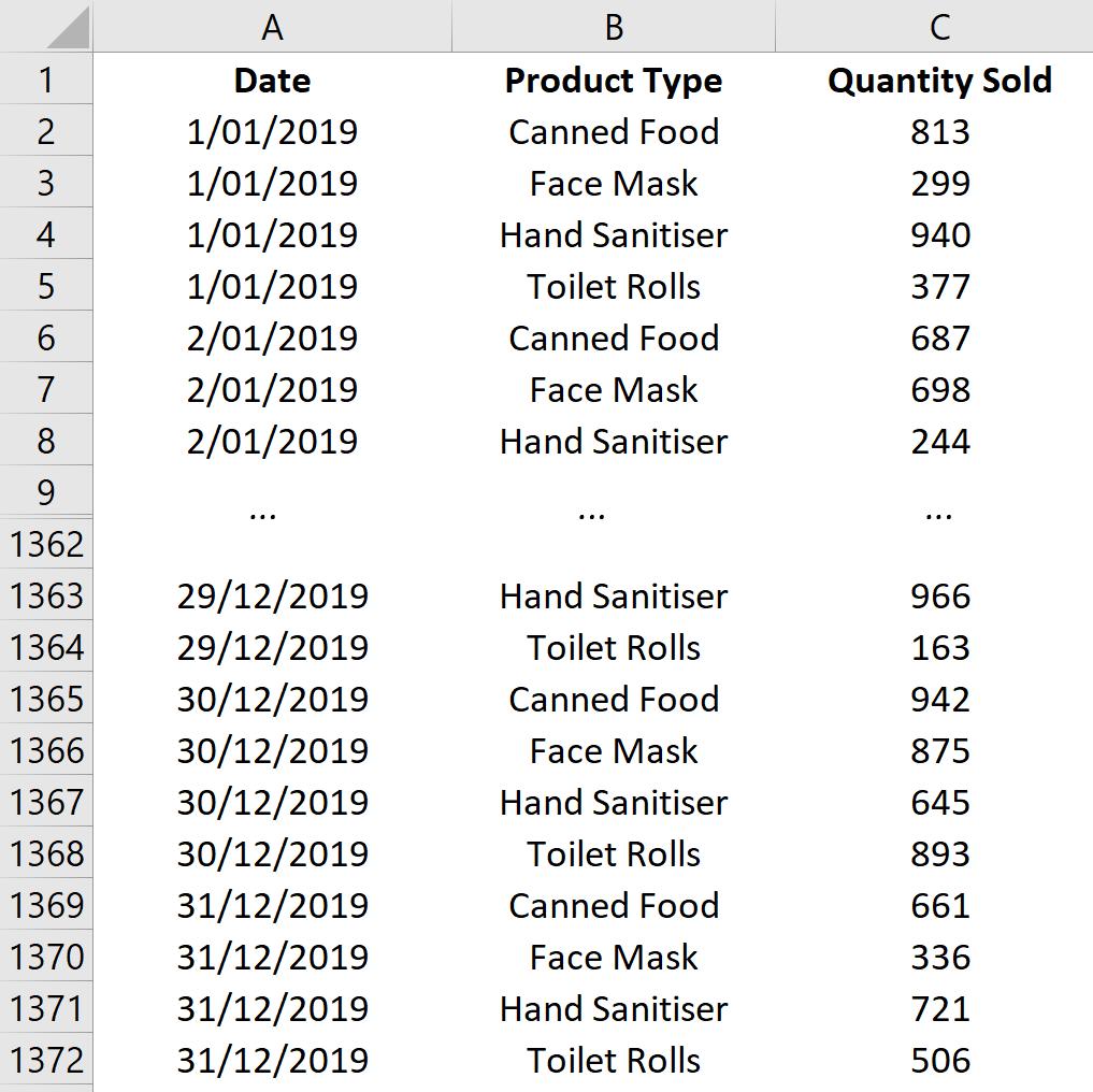
Now, let’s dive in with an example.  We have data regarding the daily sales of a few product types in a supermarket throughout 2019:

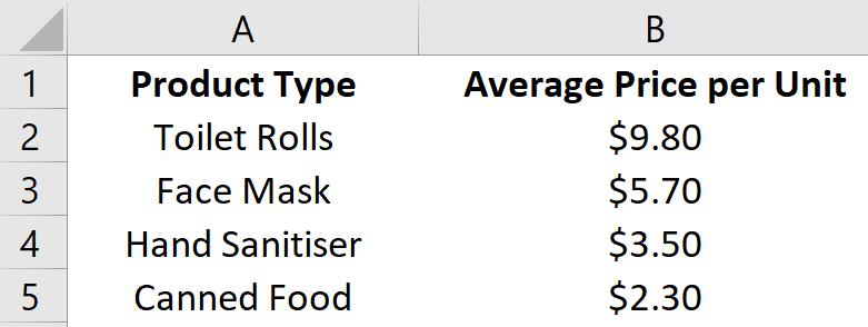
In another worksheet, we have the data for the price per unit of these products:

We want to calculate the revenue for each product in this year, equal to

Quantity Sold x Average Price per Unit.

Therefore, in the second table, we need to get total quantity sold for each product in 2019, in order to calculate this revenue.

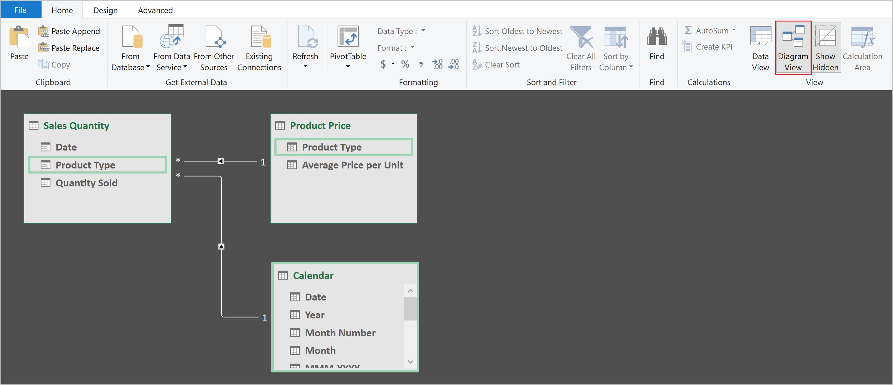
We will load the data to Power Pivot Data Model, by highlighting the whole data, going to the ‘Power Pivot’ tab on the Ribbon and clicking ‘Add to Data Model’. We rename the tables as ‘Sales Quantity’ and ‘Product Price’ respectively. We also add a Calendar Table, which will later be used in our PivotTable.

We need to define the relationships between our data tables. By switching to ‘Diagram View’ in the Home tab, we drag the ‘Product Type’ field to connect two tables, ‘Sales Quantity’ and ‘Product Price’, simultaneously, as well as the ‘Date’ field for ‘Sales Quantity’ and ‘Calendar’:

Then, switch back to the ‘Data view’, and in the ‘Product Price’ table, we apply the RELATEDTABLE function to get the ‘Quantity Sold’…but we get an error!

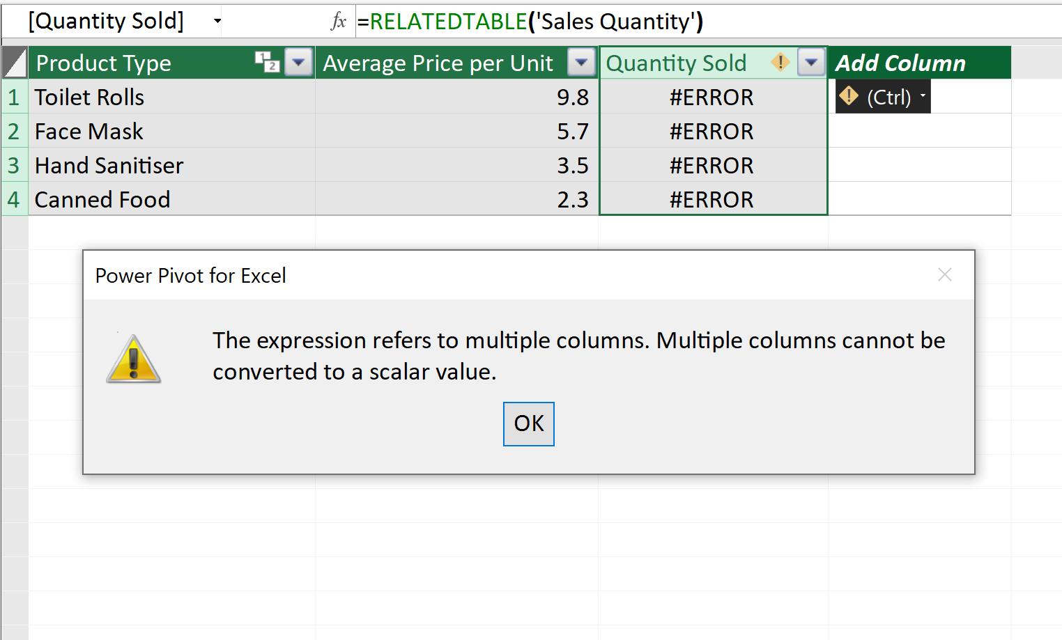
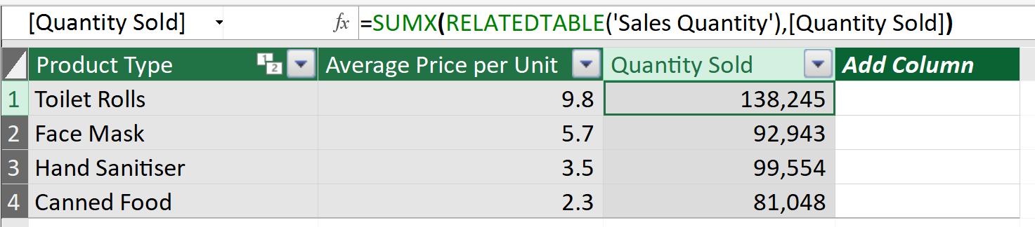
The reason is, we can’t take a table, then drop it into this cell in our data model. We need to get a count, or sum, in here. As we want to know the total number of units sold in the year, we will use the SUMX function to cover the RELATEDTABLE function thus:

=SUMX(RELATEDTABLE(‘Sales Quantity’),[Quantity Sold])

The RELATEDTABLE function will return the ‘Sales Quantity’ table, then the SUMX function will add up related data in the ‘Quantity Sold’ column:

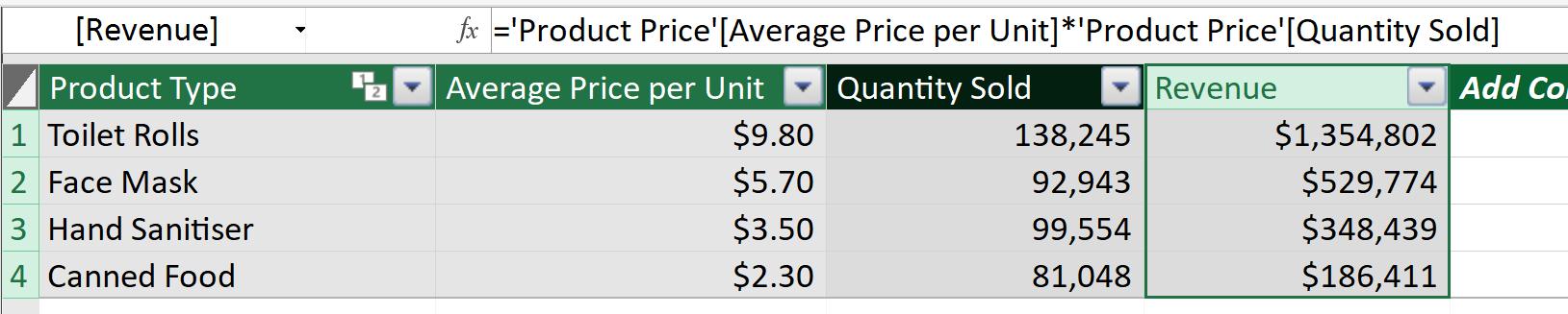
Now that we have both ‘Average Price per Unit’ and ‘Quantity Sold’ in one table, we can calculate Revenue:

=’Product Price’[Average Price per Unit]*’Product Price’[Quantity Sold]

That’s it for this week!


Stay tuned for our next post on Power Pivot in the Blog section. In the meantime, please remember we have training in Power Pivot which you can find out more about here. If you wish to catch up on past articles in the meantime, you can find all of our Past Power Pivot blogs here.