
Power Pivot Principles: Introducing the FILTER Function
14 July 2020
Welcome back to the Power Pivot Principles blog. This week, we will talk about the FILTER function in DAX.
We’ve been talking about Filters and different related filter functions in our Power Pivot Principle Blog Series, yet this is a specific FILTER function. This FILTER function returns a table that represents a subset of another table or expression. It has the following syntax:
FILTER(table, filter)
where:
- table: the table to be filtered, which can also be an expression that results in a table
- filter: a Boolean expression that is to be evaluated for each row of the table, e.g. [Sales] > 1000 or [Country] = “Australia”.
We can use the FILTER function to reduce the number of rows in the table that we are working with and use only specific data in calculations. However, this function is not to be used independently, but rather as a function that is embedded in other functions that require a table as an argument.
Consider the following example. Here, we have sales data from 2016 to 2019 for a number of stores, where they track sales by ‘Store Key’, Product, and ‘Customer Key’ viz.
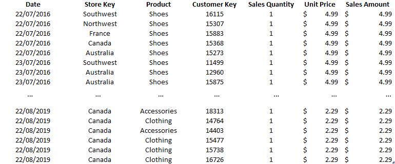
We want to see how the Australian stores sales compared to other stores, by time and by products.
We will load the data to the Power Pivot Data Model, by highlighting the whole data, going to the ‘Power Pivot’ tab on the Ribbon and clicking ‘Add to Data Model’ (this will link, rather than paste, the data in to the Data Model). We then rename the table Sales. We also add a Calendar Table, which will later be used in our PivotTable, and name it Calendar. We will also define the relationships between Sales and Calendar by switching to ‘Diagram View’ in the Home tab and dragging the Date field from one table to the other to connect them.
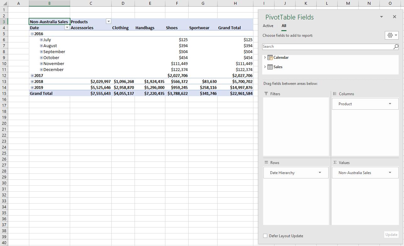
We will create a measure called ‘Non-Australia Sales’ using the FILTER function to get sales of stores other than Australia:
=SUMX(FILTER(Sales,Sales[Store Key]<>”Australia”), Sales[Sales Amount])
We then create a PivotTable, by dragging ‘Date Hierarchy’ to the Rows field, Product to the Columns field and ‘Non-Australia Sales’ to the Values field. We will then obtain a table displaying the sales of stores other than Australia, by years and by products:
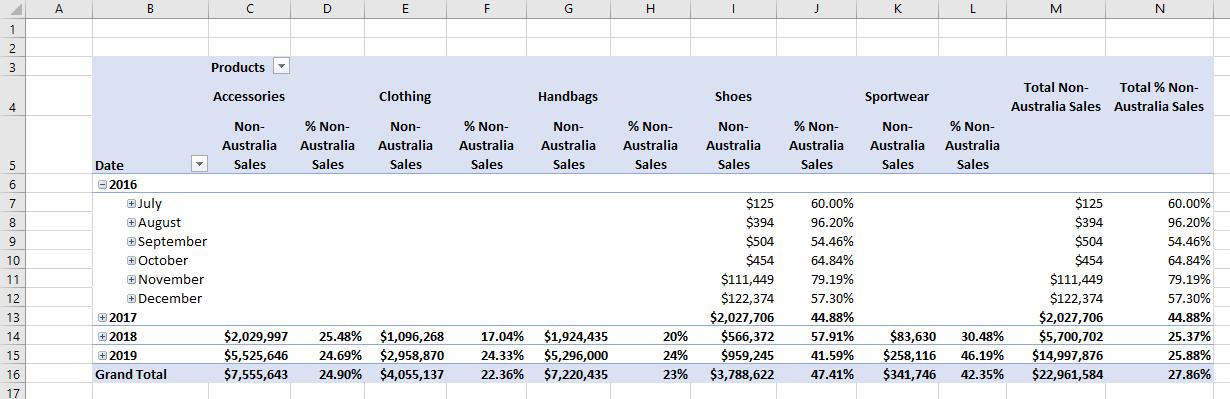
However, it is hard to get a sense from the sales number only, so we want to have a percentage of ‘Non-Australia Sales’ over total sales. Therefore, we’ll create a ‘% of Non-Australia Sales’ measure:
=DIVIDE(SUM(Sales[Sales Amount])-[Non-Australia Sales], [Non-Australia Sales])
Then, when we add ‘% of Non-Australia Sales’ to the Values field, we will create a PivotTable like the one below:
That’s it for this week!
Stay tuned for our next post on Power Pivot in the Blog section. In the meantime, please remember we have training in Power Pivot which you can find out more about >here. If you wish to catch up on past articles in the meantime, you can find all of our Past Power Pivot blogs here.