
Monday Morning Mulling: October Challenge
31 October 2016
Final Friday Fix: October Challenge Recap
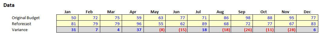
On Friday, we published a set of data comparing original budgeted numbers with their reforecast counterparts, viz.
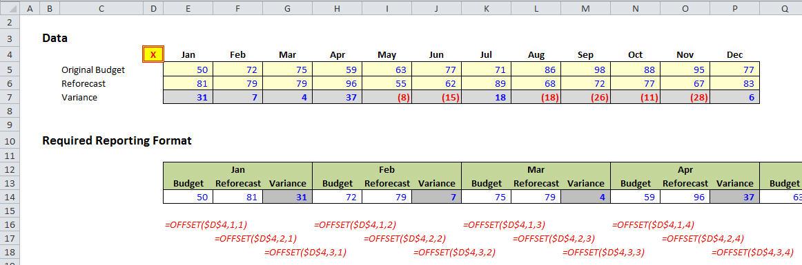
The challenge was to re-format this data for a typical management report:
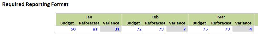
Most analysts will come up with a solution akin to the following:
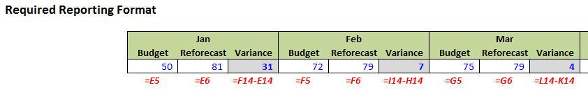
The problem is there is a different formula in each cell in the row. That means plenty of opportunities to reference the wrong cell as well as making it impossible to copy the calculation across the row.
The challenge was to create just one formula you could copy across this row that would achieve the same result.
Our Suggested Solution
You can find our solution in the attached Excel file:
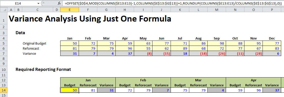
That’s right; it’s a nice simple formula:
=OFFSET($D$4,MOD(COLUMNS($E13:E13)-1,COLUMNS($E$13:$G$13))+1,ROUNDUP(COLUMNS($E13:E13)/COLUMNS($E$13:$G$13),0))
I think that might need some explanation! Let me start with the principle. Let’s look closer at the source data:
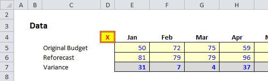
Imagine your cursor is positioned in cell D4 (the cell with the red X in it):
- To get to the January budget data, you would have to move one cell down and one column to the right
- To get to the January reforecast data, you would have to move two cells down and one column to the right
- To get to the January variance, you would have to move three cells down and one column to the right
- To get to the February budget data, you would have to move one cell down and two columns to the right
- etc.
Do you see? To get to any data in January, you have to move one column to the right; to get to any data in February you have to move two columns to the right, and so on. To get to any budget number you have to move one row down; to get to any reforecast number you have to move two rows down; to get to any variance figure, you have to move three rows down.
There’s a function that can help us with this: OFFSET (for more information, including examples and syntax, please click here). We could get a formula to work as follows:
We need the number of rows reference in the OFFSET function to go
1, 2, 3, 1, 2, 3, 1, 2, …
as the formula is copied across and we want the number of column references in the OFFSET function to go
1, 1, 1, 2, 2, 2, 3, 3, …
Using COLUMNS($E13:E13) as our counter (COLUMNS simply determines the number of columns in the cited range), we can generate both of these functions easily.
To generate the first sequence (1, 2, 3, 1, 2, 3, 1, 2, …) the MOD function (for more details and syntax please click here) works wonders:
=MOD(COLUMNS($E13:E13)-1,COLUMNS($E$13:$G$13))+1
This reverts to MOD(Counter-1,3)+1. The COLUMNS function has been used to avoid both a counter and the hard-coded value of 3. This is in accordance with our Best Practice modelling principles of Flexibility and Transparency (see >here for more details).
The ROUNDUP(value,n) function rounds the amount value up to n decimal places (so zero will be to the next whole number or integer). Therefore,
=ROUNDUP(COLUMNS($E13:E13)/COLUMNS($E$13:$G$13),0)
rounds 1/3, 2/3, 3/3, 4/3, … to the next whole number (1, 1, 1, 2, …).
Putting this all together gives us our horror formula
=OFFSET($D$4,MOD(COLUMNS($E13:E13)-1,COLUMNS($E$13:$G$13))+1,ROUNDUP(COLUMNS($E13:E13)/COLUMNS($E$13:$G$13),0))
once more. As simple as Partial Derivatives of Non-Linear Diophantine Approximation Theory!
The Final Friday Fix will return on Friday 25 November with a new Excel Challenge. In the meantime, please look out for the Daily Excel Tip on our home page and watch out for a new blog every other business workday.