
Monday Morning Mulling: May 2018 Challenge
28 May 2018
On the final Friday of each month, we set an Excel problem for you to puzzle over for the weekend. On the Monday, we publish a solution. If you think there is an alternative answer, feel free to email us. We’ll feel free to ignore you.
Final Friday Fix: May Challenge Recap
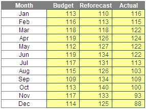
On Friday, we set up the scenario where you wanted to create a chart – say, a line chart – where you only wanted one element (line) to change. Using the following chart data,
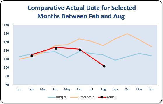
you were asked to put the following chart together with an associated Slicer:
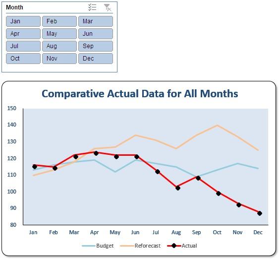
So far, so good, but the Slicer should only affect the Actual line item (in red, with the black marker in our example). For example:
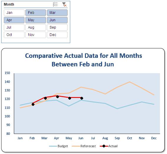
or:
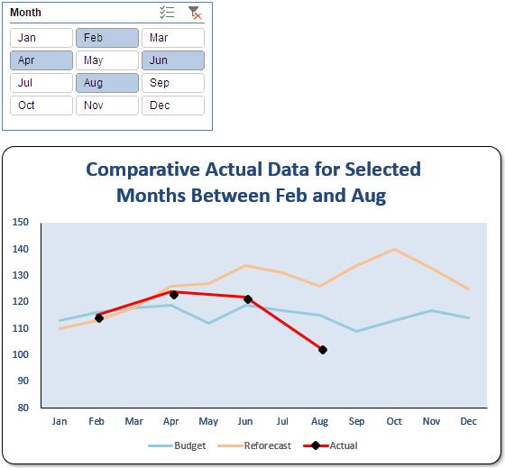
or finally:
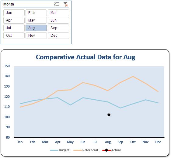
Do you see how the chart title changes automatically? That was part of the challenge too!
Suggested Solution
As always, there’s always more than one way, but here’s our approach. You can follow along with the attached Excel file.
First of all, our data has been placed in the following cells (shown just so you can follow the formulae):
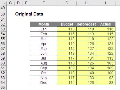
Before I play with this, I am going to highlight this entire table (cells F52:I64) and created a PivotTable (ALT + N + V), or go to the ‘Insert’ tab on the Ribbon and click on ‘PivotTables’ in the ‘Tables’ grouping) showing the months only in rows as follows:
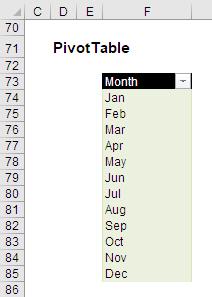
If you want a refresher on creating a PivotTable, please read our article on the topic >here. I have to have a PivotTable or a Table to create a Slicer. I tend to fall back on PivotTables (even though they are slightly more complex) as you can have one Slicer control multiple PivotTables which isn’t possible with multiple Tables.
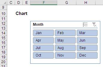
Next, I add a Slicer for the ‘Months’ field (ensure your cursor is situated in the PivotTable and then use the keyboard shortcut ALT + JT + SF, or else select ‘Insert Slicer’ from the ‘Filter’ grouping on the contextual ‘PivotTable Tools’ tab ‘Analyze’ on the Ribbon). Again, if you need a refresher on Slicers, please click here.
Since the Slicer has originated from the created PivotTable, changing the Slicer, e.g.
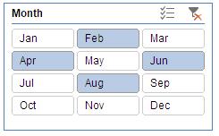
automatically manifests the same modifications in the source PivotTable, viz.

I can use this relationship to create a modified data table:
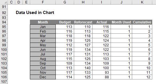
Columns F, G and H are based on the source data, but columns I:K have been calculated differently:
- Starting with column J (rather than column I), this column contains the formula:
=COUNTIF($F$74:$F$85,$F95)
- in row 95. The months only occur once in the PivotTable, so this COUNTIF function counts one (1) if the month is present in the PivotTable (i.e. the month was selected in the Slicer) and zero (0) otherwise
- Column I contains the formula
=IF(J95,I53,NA())
which references the corresponding actual data for the month provided the value in column J is TRUE, i.e. any value other than zero. Since I have already explained the only other value is 1, this formula is including the actual data if the Slicer has selected the month and puts #N/A otherwise. Whilst prima facie errors are usually discouraged in spreadsheets, in this case #N/A causes the value not to display in the chart at all.
It should be noted you might have considered the SUBTOTAL or >AGGREGATE functions instead, but as complex as they are, if the PivotTable were to be hidden, the wrong results might occur. Sometimes, simpler is better!
The cells F94:I106 are all that are required to display the chart. Simply select this range and create a line chart (ALT + N + N), or else select a lie chart from the ‘Charts’ section of the ‘Insert’ tab of the Ribbon):
- Finally, column K is required to assist with the chart title, which I haven’t yet explained. The formula here,
=SUM($J$95:$J95)*$J95
keeps a running total of all the months displayed (i.e. the first month selected is 1, the second is 2, etc.). This is useful as the number 1 relates to the earliest month and the maximum value relates to the last month selected. This latter number also represents how many months have been selected too.
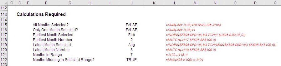
In fact, the labelling requires several preliminary calculations, viz.
Let me go through them.
The formula in cell J115, ‘All Months Selected?’,
=SUM(J95:J106)=ROWS(J95:J106)
checks to see whether the total of all of the 1’s from column I (above) equals the number of rows in the range. This can only happen if all months have a ‘1’ allocated to them, i.e. all months have been selected.
The formula in cell J116,
=SUM(J95:J106)=1
checks that one and only one month has been selected.
Cells J117 and J119 contain similar formulae. For example, the formula in the former cell,
=INDEX($F$95:$F$106,MATCH(1,$J$95:$J$106,0))
returns the name of the first month selected chronologically (the other formula identifies the last period selected). This uses the INDEX MATCH combination which we have explained previously >here.
Cells J118 and J120 use similar calculations too. The first formula
=MATCH(J117,$F$95:$F$106,0)
returns the corresponding month number (which is what the other formula does too). Therefore, the formula in cell J121,
=J120-J118+1
determines how many months would be included if all months between the first and last months had been selected. This is because the final formula in cell J122,
=MAX(K95:K106)<>J121
checks whether the number of months selected equals the number of months in total between the first and last months previously selected. If a month or more is missing, the result will be TRUE instead of FALSE.
These interim calculations are used as follows to create the chart title all in one cell:

Cell J126 contains the formula
="Comparative Actual Data for "
&IF(J115,"All Months",IF(J116,J117,IF(J122,"Selected","All")
&" Months Between "&J117&" and "&J119))
This concatenated formula will display the details required, e.g. “Comparative Actual Data for All Months or “Selected Actual Data for Aug”).
To get the formula from cell J126 into the chart itself, add a chart title, and while it is selected, click on the formula bar, type ‘=’ ad then click on cell J126. Don’t type the formula =J126 or =Example!$J$126 in. In some versions of Excel, for this to work, the cell has to be selected on the sheet for the title to become formulaically dynamic.
Simple (sort of)!
The Final Friday Fix will return on Friday 29 June with a new Excel Challenge. In the meantime, please look out for the Daily Excel Tip on our home page and watch out for a new blog every business workday.