Monday Morning Mulling: February Challenge

On the final Friday of each month, set an Excel for you to puzzle over for the weekend. On the Monday, we publish one suggested solution. No-one is stating this is the best approach, it’s just the one we selected. If you don’t like it, lump it – or contact us with your preferred solution.

Final Friday Fix: February Challenge Recap and Issue Summary

On Friday, I discussed factorials denoted by n! where

n! = n (n-1)!

i.e. n! = n (n-1) (n-2) … 3 x 2 x 1.

For example, 5! = 5 x 4 x 3 x 2 x 1 = 120. These numbers become astronomical (technical term) very quickly.

Excel has a function, FACT, which calculates factorials:

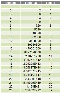
Do you see what happens from FACT(15) onwards? These numbers are expressed – and more importantly, stored – in Scientific (Exponential) notation. 15! is actually 1,307,674,368,000, although it is displayed as 1.30767E+12 and is stored as 1307674368000 (deliberately no commas), which is why its length is 13 (there are 13 digits – more precisely, characters – in the text string).

Similarly:

• 22! is actually 1,124,000,727,777,607,680,000, which is displayed by default as 1.124E+21 and is stored as 1.12400072777761E+21. This stored string has 20 characters: 15 digits (the maximum significant figures Excel can display), a decimal point and four characters for “E+21”. This means that the maximum length for a number smaller than 10¹⁰⁰ is 20 characters
• 23! is actually 25,852,016,738,884,976,640,000, which is displayed by default as 2.5852E+22 and is stored as 2.5852016738885E+22. This stored string has 19 characters. This time only 14 digits are included: this is because the 15^th number would be “0” and hence is suppressed. This is why 23! has a length of 19 rather than 22! which has a length of 20. Unlike my comment on Friday, 23! is definitely larger than 22!

Therefore, precision is of concern with larger numbers in Excel as they will only display to a maximum of 15 significant figures.

There are two more issues though.

Firstly, there’s a reason the challenge was to calculate 171!

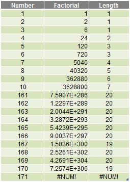
It’s the first number in the sequence Excel cannot calculate. The #NUM! error is well earned. The largest allowed positive number (which has to be calculated rather than input) is 1.7976931348623158 x 10³⁰⁸ (also denoted as 1.79769E+308). You can find out more about this and other limits here. 171! is larger than this upper bound.

Secondly, I note using numbers only will not retain precision. I need to convert the number to text so that Excel will store all the characters (that’s OK – the maximum number of characters allowed in one cell is 32,767 if I link it in from a closed workbook). The problem is, many Excel functions – including most of the useful text manipulation functions (please see here for more details) will only work with a maximum of 255 characters.

I need to get creative.

The Solution

171! is (big drum roll please)…

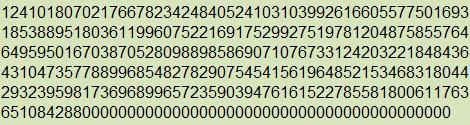
This is a screenshot straight out of the attached Excel workbook which calculates 171! as 1,241,018,070,217,667,823,424,840,524,103,103,992,616,605,577,501,693,185,388,951,803,611,996,075,221,691,752,992,751,978,120,487,585,576,464,959,501,670,387,052,809 ,889,858,690,710,767,331,242,032,218,484,364,310,473,577,889,968,548,278,290,754,541,561,964,852,153,468,318,044,293,239,598,173,696,899,657,235,903,947,616,152,278 ,558,180,061,176,365,108,428,800,000,000,000,000,000,000,000,000,000,000,000,000,000 – only without the commas!

How was this achieved? Without any VBA, I created a table in Excel to calculate the following:

1. I need to identify the largest factorial in my table (171) and multiply this by 9.99999999999999… (rounded up to 10) to work out the number of characters I need to keep in reserve, which is 171 x 10 which is 1710 (without commas). This is four characters. Given one character is already used, I need to keep three characters in reserve (this is used for the next step)
2. Since the maximum number of significant figures is 15, I need to separate my number into blocks (what I called “batches” in the model) into text strings of no more than 15 – 3 = 12 characters. This was defined as the Batch_Length
3. Define 1! as 1
4. Convert 1! (1) to a text string (“1”)
5. Now we need to calculate the next factorial
6. Calculate the character length of this string
7. Divide this length by Batch_Length (i.e. 12) rounded up to the nearest whole number. This is how many batches are needed
8. Split the text factorial into batches: Batch 1 is the final 12 characters, Batch 2 is the 24^th from last to 13^th from last digit, Batch 3 is the 36^th from last to the 25^th from last digit, and so on
9. For each batch, convert the text string back to a number simply by multiplying by the factorial you are trying to calculate (e.g. if you have just calculated 1! then multiply by two, if it is 17! then multiply by 18)
10. If the resulting number contains more than 12 characters, split the number in two: the “edited” number is the last 12 characters and the “residual” is any digits at the beginning not included
11. Add the residual from Batch n-1 to the Edited number in Batch n
12. Convert all of the numbers back to text strings
13. Concatenate the batches using the ampersand (‘&’) operator (note this cannot be done with a text function because only 255 characters are allowed and only 15 significant figures would be displayed)
14. This is the next factorial in the series
15. To calculate the next factorial in the sequence, return to Step 5 (above).

This is more complicated than it sounds (and it sounds complicated!) due to having to consider what happens if a batch in the middle of the text string starts with one or more zeros, for example. For those who would like to know more (or simply suffer with insomnia), please review the table in the attached Excel file.

Why is this Important?

Congratulations if you managed to solve this – especially if your algorithm is simpler (do share it with us!). We’re expecting many of you may have crashed and burned with this challenge.

It’s not that we are trying to create hideous challenges. It’s just that this example – and its solution highlight some key points for Excel users:

• Even when you encounter a limitation in Excel, where there’s a will there’s a way (and often a relative too)
• You need to be mindful of the degree of precision in Excel’s outputs (only 15 significant figures)
• Larger numbers may not be manipulable using Excel’s built-in functions
• Factorials (even large ones) are often used in combinatoric problems, such as selecting a subset x from a larger set y. Given x and y, the solution Excel may give may not be quite correct. This is why many statisticians often use software other than Excel.

For more tricks and tips, check out our many examples at www.sumproduct.com/thought.

The Final Friday Fix will return on Friday 31 March with a new Excel Challenge. In the meantime, please look out for the Daily Excel Tip on our home page and watch out for a new blog every other business workday.